SOLT Calibration Standards Creation

Introduction

In scikit-rf, a calibration standard is treated just as a regular one-port or two-port skrf.Network, defined by its full S-parameters. It can represent reflection, transmission, load, and even arbitrary-impedance standards. Since no additional errors are introduced in circuit modeling and fitting, this approach allows the highest calibration accuracy, and is known as a data-based standard in the terminology of VNA vendors.

However, traditionally, VNA calibration standards are defined using a circuit model with fitted coefficients. Since many such calibration kits are still being used and manufactured, especially in low-frequency applications, this necessitates the creation of their network models before they can be used in scikit-rf’s calibration routines.

This example explains network creation from coefficients given in both the HP-Agilent-Keysight format and the Rohde & Schwarz / Anritsu format. Both are essentially the same circuit model, but the latter format uses different units of measurement for an offset transmission line.

Warning

Only coaxial standards are covered by this guide. The calculation is different for waveguides. In particular, the scaling by \(\sqrt{\text{GHz}}\) for coaxial lines cannot be applied to waveguides because loss is also a function of their physical dimensions, with significant more complicated formulas. Do you have waveguide experience? If so, you can help by contributing to the doc.

Alternatives to scikit-rf Modeling

Before we begin, it’s worth pointing out some alternatives.

In scikit-rf, you are able to use any existing standard definition by its S-parameters. If you already have your standard defined as a network in other tools (e.g. in your favorite circuit simulator, or actual measurements results), you can simply export the S-parameters to Touchstone files for use in scikit-rf. Similarly, if you’re already using a data-based calibration standard, it should be possible to use its data directly. The S-parameters may be stored in device-specific file formats, consult your vendor on whether they can be exported as a Touchstone file.

Finally, for non-critical measurements below 1 GHz, sometimes one can assume the calibration standards are ideal. In scikit-rf, one can create ideal responses conveniently by defining an ideal transmission line and calling the short(), open(), match(), and thru() methods (explained in the Preparation section).

Example: HP-Agilent-Keysight Coefficient Format

After the necessary background is introduced, let’s begin.

For the purpose of this guide, we’re going to model the Keysight 85033E, 3.5 mm, 50 Ω, DC to 9 GHz calibration kit, with the following coefficients [4].

Parameter	Unit	Open	Short	Load	Thru
\(\text{C}_0\)	\(10^{−15} \text{ F}\)	49.43
\(\text{C}_1\)	\(10^{−27} \text{ F/Hz}\)	-310.1
\(\text{C}_2\)	\(10^{−36} \text{ F/Hz}^2\)	23.17
\(\text{C}_3\)	\(10^{−45} \text{ F/Hz}^3\)	-0.1597
\(\text{L}_0\)	\(10^{−12} \text{ H}\)		2.077
\(\text{L}_1\)	\(10^{−24} \text{ H/Hz}\)		-108.5
\(\text{L}_2\)	\(10^{−33} \text{ H/Hz}^2\)		2.171
\(\text{L}_3\)	\(10^{−42} \text{ H/Hz}^3\)		-0.01
Resistance	\(\Omega\)			50
Offset \(Z_0\)	\(\Omega\)	50	50	50	50
Offset Delay	ps	29.242	31.785	0	0
Offset Loss	\(\text{G}\Omega\) / s	2.2	2.36	2.3	2.3

Circuit Model

Before we start creating their network definitions, we first need to know the underlying circuit model and the meaning of these coefficients.

As this schematic shows, this is the HP-Agilent-Keysight model for a calibration standard.

The first part is an “offset” lossy transmission line, defined using three parameters: (1) A real characteristic impedance of a lossless line. This is usually the system impedance, and it matches the VNA port impedance. However, sometimes a value slightly different from the port impedance is used to model imperfections in the standard. For example, 50.209 Ω or 49.992 Ω. Also, waveguide standards use a special normalized value 1. (2) A delay - represents its electrical length, given in picoseconds, and (3) a loss. The loss is given in a somewhat unusual unit - gigaohms per second. With the three parameters, one can calculate the propagation constant (\(\gamma\)) and the complex characteristic impedance (\(Z_c\)) of the lossy line.

A shunt impedance is connected at the end of the transmission line, and models the distributed capacitance or inductance in the open or short standard. It’s given as a third-degree polynomial with four coefficients, \(y(x) = a_0 + a_1 x + a_2 x^2 + a_3 x^3\), where \(x\) is the frequency and \(a_i\) are the coefficients. For an open standard, they’re \(\text{C}_0\), \(\text{C}_1\), \(\text{C}_2\), \(\text{C}_3\), the first constant term is in femtofarad. For a short standard, they’re \(\text{L}_0\), \(\text{L}_1\), \(\text{L}_2\), \(\text{L}_3\), the first constant term is in picohenry.

Neglected Terms

The short standard may sometimes be modeled only in terms of an offset delay and offset loss, without a shunt impedance. Since the behavior of a low-inductance short circuit is reasonably linear at low frequency, one can model it as an extra delay term with acceptable accuracy.

A matched load generates little reflection, thus it’s often simply modeled as a \(Z_0\) termination, its reflection phase shift is assumed to be negligible and is given a zero offset delay.

The thru standard is sometimes modeled with an offset delay only, without loss, for two reasons: loss is negligible at low frequencies, and when the Unknown Thru calibration algorithm is used, the exact characteristics of the Thru is unimportant.

Conversely, when the Thru is used as a “flush” thru, which is the case in most traditional SOLT calibrations - port 1 and port 2 are connected directly without any adapters in the Thru step. Thus, by definition, the thru standard is completely ideal and has zero length, no modeling is required (in the table above, Keysight still gives an offset loss for Load and Thru, but both should be modeled as ideals because the listed offset delay is zero, essentially removing the offset transmission line).

Preparation

Equipped with this circuit model, we can start to model the calibration standards.

First, we need to import some library definitions, specify the frequency range of our calculation. Here, we used 1 MHz to 9 GHz, with 1001 points. You may want to adjust it for your needs. We also define an ideal_medium with a \(50 \space\Omega\) port impedance for the purpose of some future calculations.

import skrf
from skrf.media import DefinedGammaZ0
import numpy as np

freq = skrf.Frequency(1, 9000, 1001, "MHz")
ideal_medium = DefinedGammaZ0(frequency=freq, z0=50)

Ideal Responses

It’s useful to know the special case first: ideal calibration standards are easily created by calling the open(), short(), match(), and thru() methods in the ideal_medium, the first three return a 1-port network. The thru() method returns a two-port network.

ideal_open  = ideal_medium.open()
ideal_short = ideal_medium.short()
ideal_load  = ideal_medium.match()
ideal_thru  = ideal_medium.thru()

Modeling the Offset Transmission Line

To correctly model the offset transmission line, one should use the offset delay, offset loss, and offset \(Z_0\) to derive the propagation constant (\(\gamma\)) and the complex characteristic impedance (\(Z_c\)) of the lossy line. Then, an actual transmission line is defined in those terms.

The relationship between the offset line parameters and the propagation constant is given by the following equations by Keysight [1]. They’re in fact only approximate, one can obtain more accurate results by calculating the full RLCG transmission line parameters, see [3] and [4] for details. However, for practical calibration standards (1-100 ps, 1-25 Gohm/s), the author of this guide found the error is less than 0.001.

\[\begin{split}\begin{gather} \alpha l = \frac{\text{offset loss} \cdot \text{offset delay}}{2 \cdot \text{ offset }Z_0} \sqrt{\frac{f}{10^9}} \\ \beta l = 2 \pi f \cdot \text{offset delay} + \alpha l \\ \gamma l = \alpha l + j\beta l\\ Z_c = \text{offset }Z_0 + (1 - j) \frac{\text{offset loss}}{2 \cdot 2 \pi f} \sqrt{\frac{f}{10^9}} \end{gather}\end{split}\]

where \(\alpha\) is the attenuation constant of the line, in nepers per meter, \(\beta\) is the phase constant of the line, in radians per meter, \(\gamma = \alpha + j\beta\) is the propagation constant of the line, \(l\) is the length of the line, \(Z_c\) is the complex characteristic impedance of the lossy line.

Several facts need to be taken into account. First, the actual length \(l\) of the line is irrelevant: what’s being calculated here is not just \(\gamma\) but \(\gamma l\), with an implicitly defined length. Thus, if \(\gamma l\) is used as \(\gamma\), the length of the line is always set to unity (i.e. 1 meter). Next, the term \(\sqrt{\frac{f}{10^9}}\) scales the line loss from the nominal 1 GHz value to a given frequency, but this is only valid for coaxial lines, waveguides have a more complicated scaling rule. Finally, the complex characteristic impedance \(Z_c\) is different from the real characteristic impedance offset \(Z_0\). Offset \(Z_0\) does not include any losses, and it’s only used as the port impedance, while \(Z_c\) - calculated from offset \(Z_0\) and offset loss - is the actual impedance of the lossy line.

Let’s translate these formulas to code.

def offset_gamma_and_zc(offset_delay, offset_loss, offset_z0=50):
    alpha_l = (offset_loss * offset_delay) / (2 * offset_z0)
    alpha_l *= np.sqrt(freq.f / 1e9)
    beta_l = 2 * np.pi * freq.f * offset_delay + alpha_l
    gamma_l = alpha_l + 1j * beta_l
    zc = (offset_z0) + (1 - 1j) * (offset_loss / (4 * np.pi * freq.f)) * np.sqrt(freq.f / 1e9)
    return gamma_l, zc

The broadcasting feature in numpy is used here. The quantities alpha_l, beta_l, and zc are all frequency-dependent, thus they’re arrays, not scalars. But instead of looping over each frequency explicitly and adding them to an array, here, arrays are automatically created by the multiplication of a scalar and a numpy.array. We’ll continue to use this technique.

With the function offset_gamma_and_zc() defined, we can now calculate the line constants for the open and short standards by calling it.

gamma_l_open,  zc_open  = offset_gamma_and_zc(29.242e-12, 2.2e9)
gamma_l_short, zc_short = offset_gamma_and_zc(31.785e-12, 2.36e9)

At this point, we already have everything we need to know about this offset line. The other half of the task is straightforward: create a two-port network for this transmission line in scikit-rf, with a propagation constant \(\gamma l\), a characteristic impedance \(Z_c\), a port impedance \(\text{offset }Z_0=50\space\Omega\), and an unity length (1 meter, because \(\gamma l\) is used as \(\gamma\), and \(\gamma\) is measured in meters).

It’s easy but a bit confusing to perform this task in scikit-rf, it needs elaboration:

1. First, create a DefinedGammaZ0 medium with these arguments: the propagation constant gamma=gamma_l, the lossy medium impedance Z0=zc, and the VNA port impedance z0=50 (note the spelling difference between Z0 and z0). The created DefinedGammaZ0 represents a physical medium.

2. Then, an actual line with a 1-meter length is derived by calling the medium’s line() method. But now, pay attention to the arguments z0=medium.Z0 and embed=True. The argument z0 represents the line impedance. Thus, we must set z0=medium.Z0 (or zc, where medium.Z0 comes from) to get the proper line impedance we want. Finally, we must also set embed=True so that the two ports at both ends of the line are set to the port impedance (\(50\space\Omega\)) of the medium.

3. The confusing part is that in DefinedGammaZ0 class, argument z0 represents the port impedance, but in the line() method, the same z0 argument represents the line impedance instead! Also, if z0 is omitted, by default, line() uses the port impedance of the medium (not medium impedance).

In a future version, methods for specifying port and line impedances will be simplified, and it hopefully will eliminate this confusing behavior (which is why you’ll see a deprecation warning). But for now, the current implementation remains unchanged.

medium_open = DefinedGammaZ0(
    frequency=freq,
    gamma=gamma_l_open, z0=zc_open, z0_port=50
)
line_open = medium_open.line(
    d=1, unit='m'
)

medium_short = DefinedGammaZ0(
    frequency=freq,
    gamma=gamma_l_short, z0=zc_short, z0_port=50
)
line_short = medium_short.line(
    d=1, unit='m',
)

Modeling the Shunt Impedance

Then, we need to model the shunt impedance of the open and short standards. For the open standard, it’s a capacitance. For the short standard, it’s an inductance.

Both are modeled as a third-degree polynomial, as a function of frequency. In numpy, one can quickly define such a function via np.poly1d([x3, x2, x1, x0]). This is a higher-order function which accepts a list of coefficients in descending order, and returns a callable polynomial function.

After the polynomial is evaluated, we can generate the frequency-dependent capacitors and inductors. The open circuit is modeled as a series medium.capacitor() followed by an ideal medium.short(). The short circuit is modeled as a series medium.inductor() followed by an ideal medium.short().

Because the capacitor and inductor are defined with respect to the port impedance, not any particular lossy transmission line, to avoid confusions, we use ideal_medium, not medium_open or medium_short in the following examples (although the latter two are usable, they also use the port impedance).

# use ideal_medium, not medium_open and medium_short to avoid confusions.

capacitor_poly = np.poly1d([
    -0.1597 * 1e-45,
    23.17   * 1e-36,
    -310.1  * 1e-27,
    49.43   * 1e-15
])
capacitor_list = capacitor_poly(freq.f)
shunt_open = ideal_medium.capacitor(capacitor_list) ** ideal_medium.short()

inductor_poly = np.poly1d([
    -0.01   * 1e-42,
    2.171   * 1e-33,
    -108.5  * 1e-24,
    2.077   * 1e-12
])
inductor_list = inductor_poly(freq.f)
shunt_short = ideal_medium.inductor(inductor_list) ** ideal_medium.short()

For the open standard, a series medium.shunt_capacitor() terminated by a medium.open() could have also been used to get the same result. The medium.open() termination is important, because shunt_capacitor() creates a two-port network, and the other port needs to be open. Otherwise, a line terminated solely by a shunt_capacitor() produces incorrect S-parameters.

Completion

Finally, we connect these model components together, and add definitions for the ideal load and Thru, this completes our modeling.

open_std = line_open ** shunt_open
short_std = line_short ** shunt_short
load_std = ideal_medium.match()
thru_std = ideal_medium.thru()

Now you can pass these standards into scikit-rf’s calibration routines, or use the write_touchstone() method to save them on the disk for future use.

Note

Here, the open_std, short_std and load_std we generated are one-port networks, but most scikit-rf’s calibration routines expect a two-port networks as standards since they’re used in two-port calibrations. You can use the function skrf.two_port_reflect() to generate a two-port network from two one-port networks. For more information, be sure to read the SOLT calibration example in the doc.

Plotting

%matplotlib inline
import matplotlib.pyplot as plt

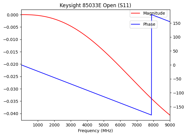
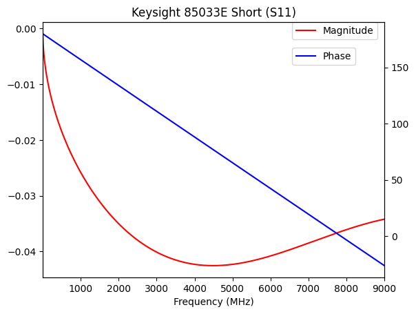
Finally, let’s take a look at the magnitudes and phase shifts of our standards.

Open

mag = plt.subplot(1, 1, 1)
plt.title("Keysight 85033E Open (S11)")
open_std.plot_s_db(color='red', label="Magnitude")
plt.legend(bbox_to_anchor=(0.73, 1), loc='upper left', borderaxespad=0)

phase = mag.twinx()
open_std.plot_s_deg(color='blue', label="Phase")
plt.legend(bbox_to_anchor=(0.73, 0.9), loc='upper left', borderaxespad=0)

<matplotlib.legend.Legend at 0x7f6a1c703af0>

Short

mag = plt.subplot(1, 1, 1)
plt.title("Keysight 85033E Short (S11)")
short_std.plot_s_db(color='red', label="Magnitude")
plt.legend(bbox_to_anchor=(0.73, 1), loc='upper left', borderaxespad=0)

phase = mag.twinx()
short_std.plot_s_deg(color='blue', label="Phase")
plt.legend(bbox_to_anchor=(0.73, 0.9), loc='upper left', borderaxespad=0)

<matplotlib.legend.Legend at 0x7f6a1c760be0>

Conclusion

As shown in the graphs above, the losses in the standards are extremely low, on the order of 0.01 dB throughout the spectrum. Meanwhile, the phase shift is what really needs compensation for. At 1 GHz, the phase shift has already reached 25 degrees or so.

Code Snippet

For convenience, you can reuse the following code snippets to generate calibration standard networks from coefficients in Keysight format.

import skrf
from skrf.media import DefinedGammaZ0
import numpy as np


def keysight_calkit_offset_line(freq, offset_delay, offset_loss, offset_z0, port_z0):
    if offset_delay or offset_loss:
        alpha_l = (offset_loss * offset_delay) / (2 * offset_z0)
        alpha_l *= np.sqrt(freq.f / 1e9)
        beta_l = 2 * np.pi * freq.f * offset_delay + alpha_l
        zc = offset_z0 + (1 - 1j) * (offset_loss / (4 * np.pi * freq.f)) * np.sqrt(freq.f / 1e9)
        gamma_l = alpha_l + beta_l * 1j

        medium = DefinedGammaZ0(frequency=freq, z0_port=offset_z0, z0=zc, gamma=gamma_l)
        offset_line = medium.line(d=1, unit='m')
        return medium, offset_line
    else:
        medium = DefinedGammaZ0(frequency=freq, z0=offset_z0)
        line = medium.line(d=0)
        return medium, line


def keysight_calkit_open(freq, offset_delay, offset_loss, c0, c1, c2, c3, offset_z0=50, port_z0=50):
    medium, line = keysight_calkit_offset_line(freq, offset_delay, offset_loss, offset_z0, port_z0)
    # Capacitance is defined with respect to the port impedance offset_z0, not the lossy
    # line impedance. In scikit-rf, the return values of `shunt_capacitor()` and `medium.open()`
    # methods are (correctly) referenced to the port impedance.
    if c0 or c1 or c2 or c3:
        poly = np.poly1d([c3, c2, c1, c0])
        capacitance = medium.shunt_capacitor(poly(freq.f)) ** medium.open()
    else:
        capacitance = medium.open()
    return line ** capacitance


def keysight_calkit_short(freq, offset_delay, offset_loss, l0, l1, l2, l3, offset_z0=50, port_z0=50):
    # Inductance is defined with respect to the port impedance offset_z0, not the lossy
    # line impedance. In scikit-rf, the return values of `inductor()` and `medium.short()`
    # methods are (correctly) referenced to the port impedance.
    medium, line = keysight_calkit_offset_line(freq, offset_delay, offset_loss, offset_z0, port_z0)
    if l0 or l1 or l2 or l3:
        poly = np.poly1d([l3, l2, l1, l0])
        inductance = medium.inductor(poly(freq.f)) ** medium.short()
    else:
        inductance = medium.short()
    return line ** inductance


def keysight_calkit_load(freq, offset_delay=0, offset_loss=0, offset_z0=50, port_z0=50):
    medium, line = keysight_calkit_offset_line(freq, offset_delay, offset_loss, offset_z0, port_z0)
    load = medium.match()
    return line ** load


def keysight_calkit_thru(freq, offset_delay=0, offset_loss=0, offset_z0=50, port_z0=50):
    medium, line = keysight_calkit_offset_line(freq, offset_delay, offset_loss, offset_z0, port_z0)
    thru = medium.thru()
    return line ** thru


freq = skrf.Frequency(1, 9000, 1001, "MHz")
open_std = keysight_calkit_open(
    freq,
    offset_delay=29.242e-12, offset_loss=2.2e9,
    c0=49.43e-15, c1=-310.1e-27, c2=23.17e-36, c3=-0.1597e-45
)
short_std = keysight_calkit_short(
    freq,
    offset_delay=31.785e-12, offset_loss=2.36e9,
    l0=2.077e-12, l1=-108.5e-24, l2=2.171e-33, l3=-0.01e-42
)
load_std = keysight_calkit_load(freq)
thru_std = keysight_calkit_thru(freq)

# hypothetically, the S-parameters of the same 50-ohm short standard as measured by a 75-ohm VNA
short_std_50_on_75 = keysight_calkit_short(
    freq,
    offset_delay=31.785e-12, offset_loss=2.36e9,
    l0=2.077e-12, l1=-108.5e-24, l2=2.171e-33, l3=-0.01e-42,
    offset_z0=50, port_z0=75
)
# hypothetically, a 49.992-ohm short standard for use with a 50-ohm VNA
short_std_49_on_50 = keysight_calkit_short(
    freq,
    offset_delay=31.785e-12, offset_loss=2.36e9,
    l0=2.077e-12, l1=-108.5e-24, l2=2.171e-33, l3=-0.01e-42,
    offset_z0=49.992, port_z0=50
)
# hypothetically, a 75-ohm short standard for a 75-ohm VNA
short_std_75 = keysight_calkit_short(
    freq,
    offset_delay=31.785e-12, offset_loss=2.36e9,
    l0=2.077e-12, l1=-108.5e-24, l2=2.171e-33, l3=-0.01e-42,
    offset_z0=75, port_z0=75
)

Example: Rohde & Schwarz / Anritsu Coefficient Format

On Rohde & Schwarz and Anritsu VNAs, a slightly different format is used to define the coefficients. Here’s an example of a Maury Microwave 8050CK10, a 3.5 mm, DC to 26.5 GHz calibration kit defined in Rohde & Schwartz’s format [5].

Parameter	Unit	Open	Short	Load	Thru
\(\text{C}_0\)	\(10^{−15} \text{ F}\)	62.54
\(\text{C}_1\)	\(10^{−15} \text{ F/GHz}\)	1284.0
\(\text{C}_2\)	\(10^{−15} \text{ F/GHz}^2\)	107.6
\(\text{C}_3\)	\(10^{−15} \text{ F/GHz}^3\)	-1.886
\(\text{L}_0\)	\(10^{−12} \text{ H}\)		0
\(\text{L}_1\)	\(10^{−12} \text{ H/GHz}\)		0
\(\text{L}_2\)	\(10^{−12} \text{ H/GHz}^2\)		0
\(\text{L}_3\)	\(10^{−12} \text{ H/GHz}^3\)		0
Resistance	\(\Omega\)			50
Offset Length	mm	4.344	5.0017	0	17.375
Offset Loss	\(\text{dB / }\sqrt{\text{GHz}}\)	0.0033	0.0038	0	0.0065

Modeling the Offset Transmission Line

As shown, it’s essentially the same circuit model, the only difference is that the offset transmission line is defined in different units of measurements: offset delay is defined as a physical length instead of a time delay, offset loss is defined in decibel, the offset \(Z_0\) is defined to be \(50 \space\Omega\) and unlisted.

We can reuse the same calculations in the Keysight model after a simple unit conversion using these equations [2].

\[\begin{split}\begin{gather} \text{D'} = \frac{D \cdot \sqrt{\epsilon_r}}{c_0} \\ \text{L'} = \frac{L \cdot Z_0}{D' \cdot 20 \log_{10}{(e)}} \end{gather}\end{split}\]

where \(D\) and \(L\) are the offset length (meter) and offset loss (\(\text{dB / }\sqrt{\text{GHz}}\)) in the R&S model, \(D'\) and \(L'\) are the offset delay (second) and offset loss (\(\Omega\) / s) in Keysight’s model, \(\epsilon_r\) is the dielectric constant, it’s air by definition, thus \(\epsilon_r = 1\), and \(c_0\) is the speed of light. The term \(20 \log_{10}{(e)}\) is a conversion from decibel to neper.

def rs_to_keysight(rs_offset_length, rs_offset_loss, offset_z0=50):
    offset_delay = rs_offset_length / skrf.constants.c
    offset_loss = skrf.mathFunctions.db_2_np(rs_offset_loss * offset_z0 / offset_delay)
    return offset_delay, offset_loss

After unit conversion, we can define standards just like how calibration standards in Keysight-style coefficients are defined.

offset_delay, offset_loss = rs_to_keysight(4.344e-3, 0.0033)
gamma_l, zc = offset_gamma_and_zc(offset_delay, offset_loss)
medium_open = DefinedGammaZ0(
    frequency=freq,
    gamma=gamma_l, z0=zc, z0_port=50
)
line_open = medium_open.line(
    d=1, unit='m'
)

offset_delay, offset_loss = rs_to_keysight(5.0017e-3, 0.0038)
gamma_l, zc = offset_gamma_and_zc(offset_delay, offset_loss)
medium_short = DefinedGammaZ0(
    frequency=freq,
    gamma=gamma_l, z0=zc, z0_port=50
)
line_short = medium_short.line(
    d=1, unit='m'
)

offset_delay, offset_loss = rs_to_keysight(17.375e-3, 0.0065)
gamma_l, zc = offset_gamma_and_zc(offset_delay, offset_loss)
medium_thru = DefinedGammaZ0(
    frequency=freq,
    gamma=gamma_l, z0=zc, z0_port=50
)
line_thru = medium_thru.line(
    d=1, unit='m'
)

Modeling the Shunt Impedance

The definition of shunt impedance is identical to the Keysight format.

But, beware of the units used for the capacitance and inductance! In the given table, the capacitances are given in \(10^{−15} \text{ F}\), \(10^{−15} \text{ F/GHz}\), \(10^{−15} \text{ F/GHz}^2\), and \(10^{−15} \text{ F/GHz}^3\). For Keysight and Anritsu VNAs, they’re given in \(10^{-15} \text{ F}\), \(10^{-27} \text{ F/Hz}\), \(10^{-36} \text{ F/Hz}^2\) and \(10^{-45} \text{ F/Hz}^3\). Inductance units have the same differences. Always double-check the units before start modeling. To convert the units from the first to the second format, multiply \(x_1\), \(x_2\) and \(x_3\) by 1000 (don’t change the constant term \(x_0\)). For consistency, we’ll use the second format in the code.

Since the inductance in the short standard is neglected, only the capacitance in the open standard is modeled, the short is modeled as ideal.

capacitor_poly = np.poly1d([
    -0.001886 * 1000e-45,
     0.1076   * 1000e-36,
    -1.284    * 1000e-27,
    62.54     * 1e-15
])
capacitor_open = capacitor_poly(freq.f)
shunt_open = ideal_medium.shunt_capacitor(capacitor_open) ** ideal_medium.open()
# or: shunt_open = ideal_medium.capacitor(capacitor_open) ** ideal_medium.short()
# see the Keysight example for explanation.

shunt_short = ideal_medium.short()

Completion

Finally, we connect these model components together.

open_std = line_open ** shunt_open
short_std = line_short ** shunt_short
load_std = ideal_medium.match()
thru_std = line_thru

Plotting

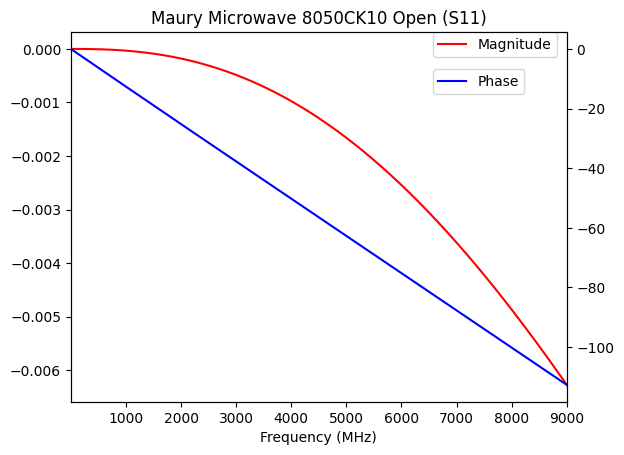
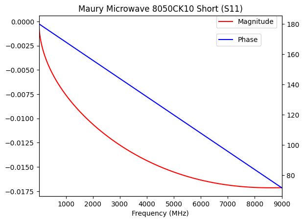
Again, let’s examine the behaviors of the finished standards.

Open

mag = plt.subplot(1, 1, 1)
plt.title("Maury Microwave 8050CK10 Open (S11)")
open_std.plot_s_db(color='red', label="Magnitude")
plt.legend(bbox_to_anchor=(0.73, 1), loc='upper left', borderaxespad=0)

phase = mag.twinx()
open_std.plot_s_deg(color='blue', label="Phase")
plt.legend(bbox_to_anchor=(0.73, 0.9), loc='upper left', borderaxespad=0)

<matplotlib.legend.Legend at 0x7f6a1c538c10>

Short

mag = plt.subplot(1, 1, 1)
plt.title("Maury Microwave 8050CK10 Short (S11)")
short_std.plot_s_db(color='red', label="Magnitude")
plt.legend(bbox_to_anchor=(0.73, 1), loc='upper left', borderaxespad=0)

phase = mag.twinx()
short_std.plot_s_deg(color='blue', label="Phase")
plt.legend(bbox_to_anchor=(0.73, 0.9), loc='upper left', borderaxespad=0)

<matplotlib.legend.Legend at 0x7f6a1c483610>

Thru

mag = plt.subplot(1, 1, 1)
plt.title("Maury Microwave 8050CK10 Thru (S21)")
thru_std.s21.plot_s_db(color='red', label="Magnitude")
plt.legend(bbox_to_anchor=(0.73, 1), loc='upper left', borderaxespad=0)

phase = mag.twinx()
thru_std.s21.plot_s_deg(color='blue', label="Phase")
plt.legend(bbox_to_anchor=(0.73, 0.9), loc='upper left', borderaxespad=0)

<matplotlib.legend.Legend at 0x7f6a1c37ece0>

Conclusion

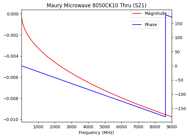
The results are similar to the Keysight calibration standards. The S21 graph for the Thru standard explains why adding an electrical delay sometimes can serve as a crude but usable calibration method (“port extension”) for VNA measurements. Again, losses are extremely low, phase shift is the source of non-ideal properties in the standards.

Code Snippet

For convenience, you can reuse the following code snippet to generate calibration standard networks from coefficients in Rhode & Swartz and Anritsu format.

import skrf
from skrf.media import DefinedGammaZ0
import numpy as np


def rs_to_keysight(rs_offset_length, rs_offset_loss, offset_z0=50):
    offset_delay = rs_offset_length / skrf.constants.c
    offset_loss = skrf.mathFunctions.db_2_np(rs_offset_loss * offset_z0 / offset_delay)
    return offset_delay, offset_loss


def rs_calkit_offset_line(freq, rs_offset_length, rs_offset_loss, offset_z0, port_z0):
    if rs_offset_length or rs_offset_loss:
        offset_delay, offset_loss = rs_to_keysight(rs_offset_length, rs_offset_loss)

        alpha_l = (offset_loss * offset_delay) / (2 * offset_z0)
        alpha_l *= np.sqrt(freq.f / 1e9)
        beta_l = 2 * np.pi * freq.f * offset_delay + alpha_l
        zc = offset_z0 + (1 - 1j) * (offset_loss / (4 * np.pi * freq.f)) * np.sqrt(freq.f / 1e9)
        gamma_l = alpha_l + beta_l * 1j

        medium = DefinedGammaZ0(frequency=freq, z0_port=offset_z0, z0=zc, gamma=gamma_l)
        offset_line = medium.line(d=1, unit='m')
        return medium, offset_line
    else:
        medium = DefinedGammaZ0(frequency=freq, z0=offset_z0)
        line = medium.line(d=0)
        return medium, line


def rs_calkit_open(freq, offset_length, offset_loss, c0, c1, c2, c3, offset_z0=50, port_z0=50):
    # Capacitance is defined with respect to the port impedance offset_z0, not the lossy
    # line impedance. In scikit-rf, the return values of `shunt_capacitor()` and `medium.open()`
    # methods are (correctly) referenced to the port impedance.
    medium, line = rs_calkit_offset_line(freq, offset_length, offset_loss, offset_z0, port_z0)
    if c0 or c1 or c2 or c3:
        poly = np.poly1d([c3, c2, c1, c0])
        capacitance = medium.shunt_capacitor(poly(freq.f)) ** medium.open()
    else:
        capacitance = medium.open()
    return line ** capacitance


def rs_calkit_short(freq, offset_length, offset_loss, l0, l1, l2, l3, offset_z0=50, port_z0=50):
    # Inductance is defined with respect to the port impedance offset_z0, not the lossy
    # line impedance. In scikit-rf, the return values of `inductor()` and `medium.short()`
    # methods are (correctly) referenced to the port impedance.
    medium, line = rs_calkit_offset_line(freq, offset_length, offset_loss, offset_z0, port_z0)
    if l0 or l1 or l2 or l3:
        poly = np.poly1d([l3, l2, l1, l0])
        inductance = medium.inductor(poly(freq.f)) ** medium.short()
    else:
        inductance = medium.short()
    return line ** inductance


def rs_calkit_load(freq, offset_length=0, offset_loss=0, offset_z0=50, port_z0=50):
    medium, line = rs_calkit_offset_line(freq, offset_length, offset_loss, offset_z0, port_z0)
    load = medium.match()
    return line ** load


def rs_calkit_thru(freq, offset_length=0, offset_loss=0, offset_z0=50, port_z0=50):
    medium, line = rs_calkit_offset_line(freq, offset_length, offset_loss, offset_z0, port_z0)
    thru = medium.thru()
    return line ** thru


freq = skrf.Frequency(1, 9000, 1001, "MHz")
open_std = rs_calkit_open(
    freq,
    offset_length=4.344e-3, offset_loss=0.0033,
    # Due to unit differences, the numerical values of c1, c2 and c3
    # must be multiplied by 1000 from the R&S datasheet value. For
    # Anritsu, this is not needed. Check the units on your datasheet!
    c0=62.54     * 1e-15,
    c1=-1.284    * 1000e-27,
    c2=0.1076    * 1000e-36,
    c3=-0.001886 * 1000e-45
)
short_std = rs_calkit_short(
    freq,
    offset_length=5.0017e-3, offset_loss=0.0038,
    l0=0, l1=0, l2=0, l3=0
)
load_std = rs_calkit_load(freq)
thru_std = rs_calkit_thru(
    freq,
    offset_length=17.375e-3, offset_loss=0.0065
)

# hypothetically, the S-parameters of the same 50-ohm short standard as measured by a 75-ohm VNA
short_std_50_on_75 = rs_calkit_short(
    freq,
    offset_length=5.0017e-3, offset_loss=0.0038,
    l0=0, l1=0, l2=0, l3=0,
    offset_z0=50, port_z0=75
)
# hypothetically, a 49.992-ohm short standard for use with a 50-ohm VNA
short_std_49_on_50 = rs_calkit_short(
    freq,
    offset_length=5.0017e-3, offset_loss=0.0038,
    l0=0, l1=0, l2=0, l3=0,
    offset_z0=49.992, port_z0=50
)
# hypothetically, a 75-ohm short standard for a 75-ohm VNA
short_std_75 = rs_calkit_short(
    freq,
    offset_length=5.0017e-3, offset_loss=0.0038,
    l0=0, l1=0, l2=0, l3=0,
    offset_z0=75, port_z0=75
)

References

[1]: Specifying Calibration Standards and Kits for Agilent Vector Network Analyzers. See Equation 36, 37 for the propagation constant formulas of the offset transmission line.

[2]: METAS VNA Tools II - Math Reference V2.1. See Page 26, 27 for formulas of the Keysight and R&S coefficients. The Keysight formulas are equivalent to [1].

[3]: S-Parameters for Signal Integrity, Peter J. Pupalaikis. Page 481.

[4]: Effect of Loss on VNA Calibration Standards. Source of the Keysight 85033E example.

[5]: Maury Microwave 3.5mm Coaxial Calibration Kit User Guide. Source of the Maury Microwave 8050CK10 example. The coefficients of this calibration kit are given in multiple formats (Anritsu, Keysight, and R&S). You can compare and contrast their differences.