Ex4: Passivity Evaluation and Enforcement

To demonstrate the passivity evaluation and enforcement features of the vector fitting class, the ring slot example 2-port is used, once again. Have a look at the other vector fitting example notebooks for more general explanations of the fitting process.

import skrf
import numpy as np
import matplotlib.pyplot as mplt

# load and fit the ring slot network with 3 poles
nw = skrf.data.ring_slot
vf = skrf.VectorFitting(nw)
vf.vector_fit(n_poles_real=3, n_poles_cmplx=0)

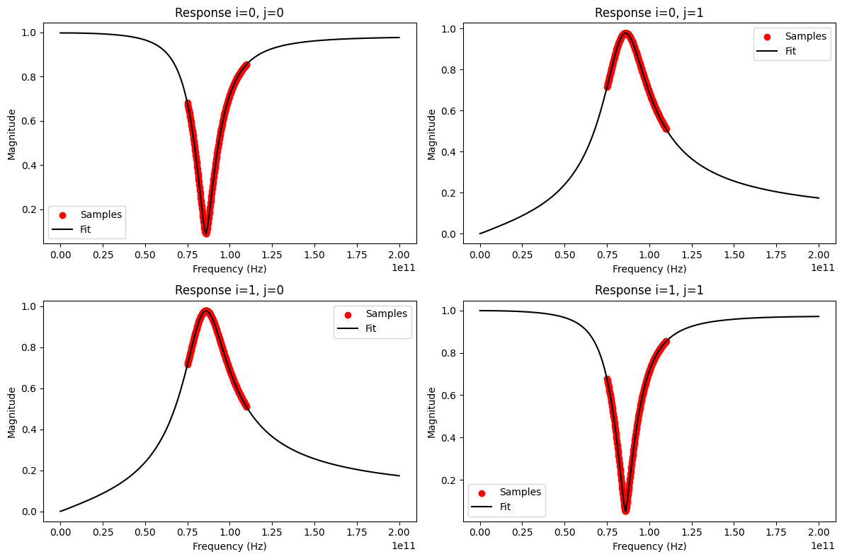
# plot fitting results
freqs = np.linspace(0, 200e9, 201)
fig, ax = mplt.subplots(2, 2)
fig.set_size_inches(12, 8)
vf.plot_s_mag(0, 0, freqs=freqs, ax=ax[0][0]) # s11
vf.plot_s_mag(0, 1, freqs=freqs, ax=ax[0][1]) # s12
vf.plot_s_mag(1, 0, freqs=freqs, ax=ax[1][0]) # s21
vf.plot_s_mag(1, 1, freqs=freqs, ax=ax[1][1]) # s22
fig.tight_layout()
mplt.show()

/tmp/ipykernel_8216/1560071222.py:8: UserWarning: The fitted network is passive, but the vector fit is not passive. Consider running `passivity_enforce()` to enforce passivity before using this model.
  vf.vector_fit(n_poles_real=3, n_poles_cmplx=0)

The fitting result looks fine, but a UserWarning about a non-passive vector fit was printed. Before investigating this issue, let’s check the RMS error:

vf.get_rms_error()

0.0038558033974603256

An RMS error of less than 0.05 usually indicates a good fit and confirms our optical inspection. But what about the passivity of the fitted model?

vf.is_passive()

False

Why is the model not passive? Wasn’t the original data of the ring slot representing a passive network?

nw.is_passive()

True

The network data was passive, but the vector fitted model is not. Let’s investigate (and correct?) the problem some more.

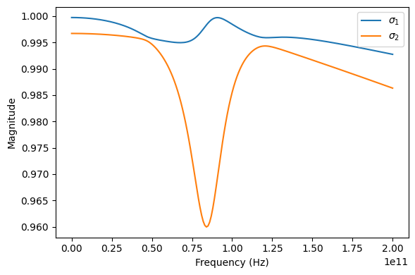
# plot singular values of vector fitted scattering matrix
freqs = np.linspace(0, 200e9, 201)
fig, ax = mplt.subplots(1, 1)
fig.set_size_inches(6, 4)
vf.plot_s_singular(freqs=freqs, ax=ax)
fig.tight_layout()
mplt.show()

One of the singular values of the fitted scattering matrix is greater than 1 at some frequencies. This indeed indicates a non-passive model. For further analysis, you can get a list of all frequency bands with passivity violations:

vf.passivity_test()

array([[0.00000000e+00, 2.78120033e+10],
       [8.43130648e+10, 9.83113388e+10]])

The network is not passive in two frequency bands: From dc to about 27.8 GHz, and from 84.3 GHz to 98.5 GHz. Luckily, passivity can be enforced to obtain passive vector fitted model:

vf.passivity_enforce()

After passivity enforcement, the network should be passive at all frequencies. Let’s check ourselves:

vf.is_passive()

True

vf.passivity_test()

array([], dtype=float64)

# plot singular values of vector fitted scattering matrix
freqs = np.linspace(0, 200e9, 201)
fig, ax = mplt.subplots(1, 1)
fig.set_size_inches(6, 4)
vf.plot_s_singular(freqs=freqs, ax=ax)
fig.tight_layout()
mplt.show()

Alright, the model is finally passive. But does it still fit the original network data?

# plot fitting results again after passivity enforcement
freqs = np.linspace(0, 200e9, 201)
fig, ax = mplt.subplots(2, 2)
fig.set_size_inches(12, 8)
vf.plot_s_mag(0, 0, freqs=freqs, ax=ax[0][0]) # s11
vf.plot_s_mag(0, 1, freqs=freqs, ax=ax[0][1]) # s12
vf.plot_s_mag(1, 0, freqs=freqs, ax=ax[1][0]) # s21
vf.plot_s_mag(1, 1, freqs=freqs, ax=ax[1][1]) # s22
fig.tight_layout()
mplt.show()

In addition to the visual inspection, let’s check the RMS error again:

vf.get_rms_error()

0.0041624780938994445

Yes, the model still fits the original data very well and the differences to the first non-passive fit from above are insignificant: the rms error is still very low.