Ex2: Measured 190 GHz Active 2-Port

The Vector Fitting feature is demonstrated using a 2-port S-matrix of an active circuit measured from 140 GHz to 220 GHz. Additional explanations and background information can be found in the Vector Fitting tutorial.

import skrf
import numpy as np
import matplotlib.pyplot as mplt

This example is a lot more tricky to fit, because the responses contain a few “bumps” and noise from the measurement. In such a case, finding a good number of initial poles can take a few iterations.

Load the Network from a Touchstone file and create the Vector Fitting instance:

nw = skrf.network.Network('./190ghz_tx_measured.S2P')
vf = skrf.VectorFitting(nw)

First attempt: Perform the fit using 4 real poles and 4 complex-conjugate poles: (Note: In a previous version of this example, the order of the two attempts was reversed. Also see the comment at the end.)

vf.vector_fit(n_poles_real=4, n_poles_cmplx=4)

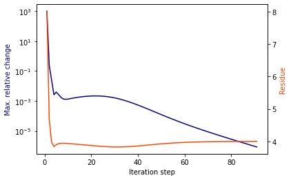
The function plot_convergence() can be helpful to examine the convergence and see if something was going wrong.

vf.plot_convergence()

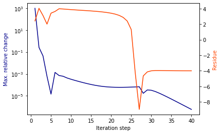
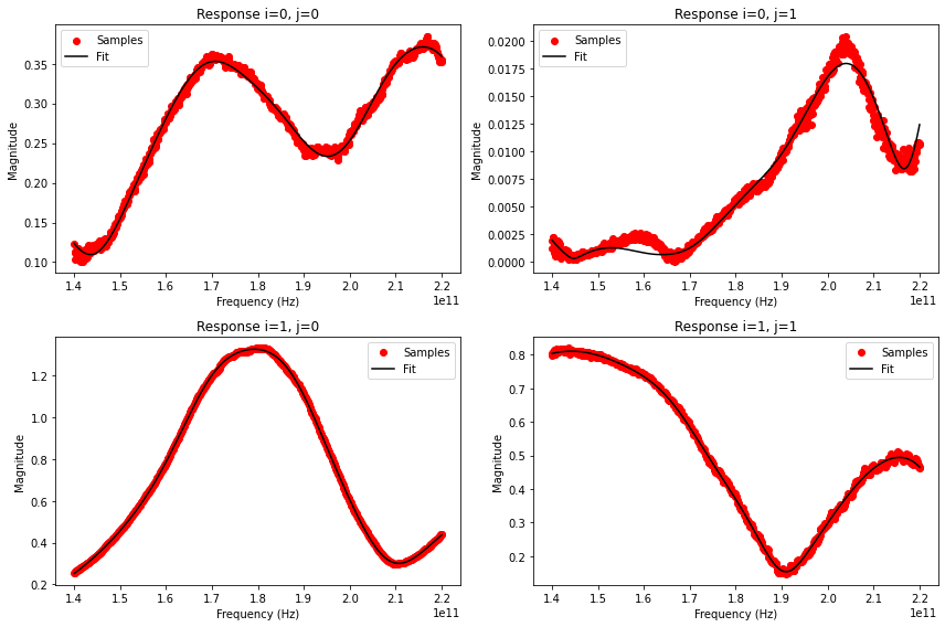
Checking the results by comparing the model responses to the original sampled data indicates a successful fit, which is also indicated by a small rms error (less than 0.05):

vf.get_rms_error()

0.014738359454393082

# plot frequency responses
fig, ax = mplt.subplots(2, 2)
fig.set_size_inches(12, 8)
vf.plot_s_mag(0, 0, ax=ax[0][0]) # s11
vf.plot_s_mag(0, 1, ax=ax[0][1]) # s12
vf.plot_s_mag(1, 0, ax=ax[1][0]) # s21
vf.plot_s_mag(1, 1, ax=ax[1][1]) # s22
fig.tight_layout()
mplt.show()

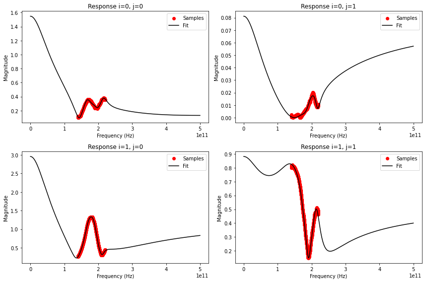
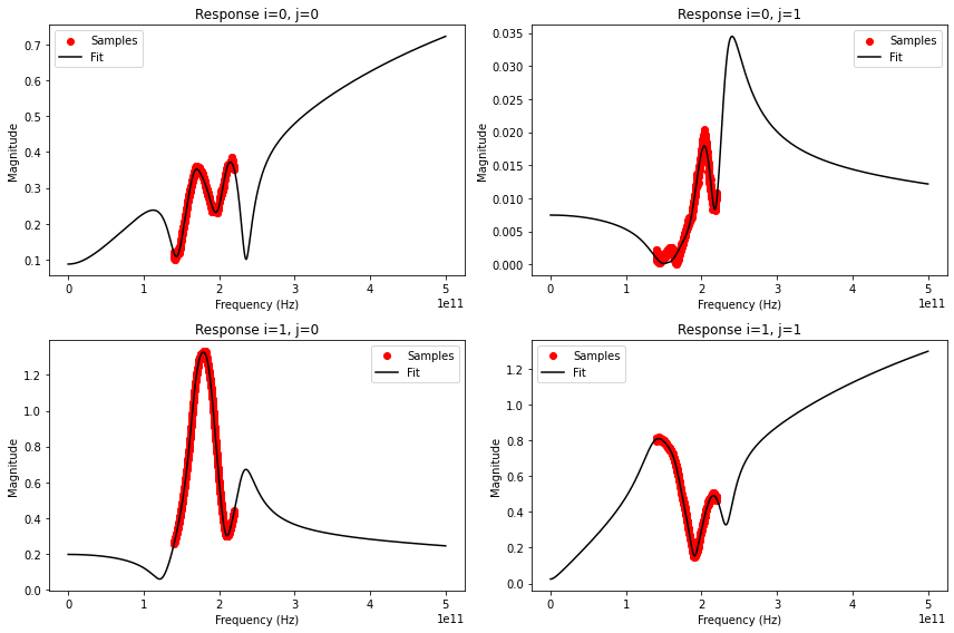
It is a good idea to also check the model response well outside the original frequency range.

freqs = np.linspace(0, 500e9, 501) # plot model response from dc to 500 GHz
fig, ax = mplt.subplots(2, 2)
fig.set_size_inches(12, 8)
vf.plot_s_mag(0, 0, freqs=freqs, ax=ax[0][0]) # s11
vf.plot_s_mag(0, 1, freqs=freqs, ax=ax[0][1]) # s12
vf.plot_s_mag(1, 0, freqs=freqs, ax=ax[1][0]) # s21
vf.plot_s_mag(1, 1, freqs=freqs, ax=ax[1][1]) # s22
fig.tight_layout()
mplt.show()

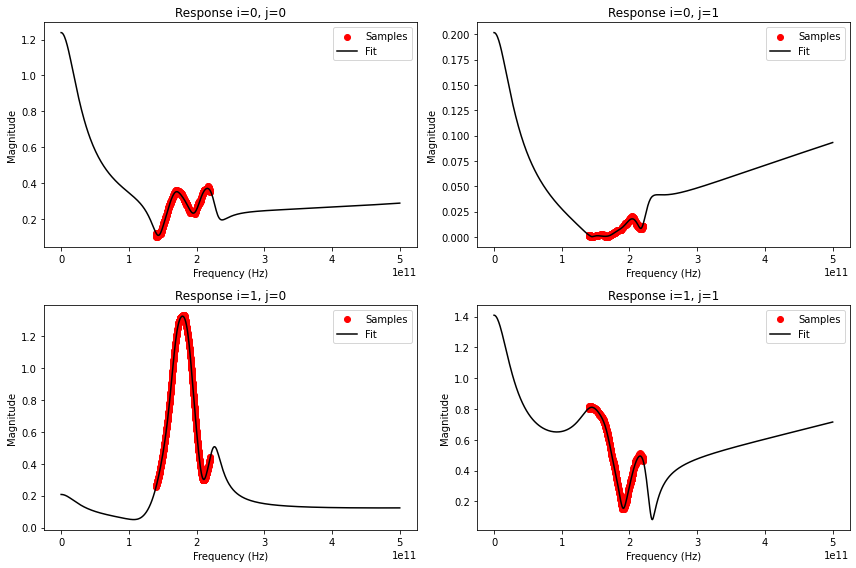
Second attempt: Maybe an even better fit without that large dc “spike” can be achieved, so let’s try again. Unwanted spikes at frequencies outside the fitting band are often caused by unnecessary or badly configured poles. Predictions about the fitting quality outside the fitting band are somewhat speculative and are not exactly controllable without additional samples at those frequencies. Still, let’s try to decrease the number of real starting poles to 3 and see if the dc spike is removed: (Note: One could also reduce the real poles and/or increase the complex-conjugate poles. Also see the comment at the end.)

vf.vector_fit(n_poles_real=3, n_poles_cmplx=4)
vf.plot_convergence()

This fit took more iterations, but it converged nevertheless and it matches the network data very well inside the fitting band. Again, a small rms error is achieved:

vf.get_rms_error()

0.015223407583253244

fig, ax = mplt.subplots(2, 2)
fig.set_size_inches(12, 8)
vf.plot_s_mag(0, 0, freqs=freqs, ax=ax[0][0]) # s11
vf.plot_s_mag(0, 1, freqs=freqs, ax=ax[0][1]) # s12
vf.plot_s_mag(1, 0, freqs=freqs, ax=ax[1][0]) # s21
vf.plot_s_mag(1, 1, freqs=freqs, ax=ax[1][1]) # s22
fig.tight_layout()
mplt.show()

This looks good, so let’s export the model as a SPICE subcircuit. For example:

vf.write_spice_subcircuit_s('/home/vinc/Desktop/190ghz_tx.sp')

The subcircuit can then be simulated in SPICE with the same AC simulation setup as in the ring slot example:

Comment on starting poles:

During the pole relocation process (first step in the fitting process), the starting poles are sucessively moved to frequencies where they can best match all target responses. Additionally, the type of poles can change from real to complex-conjugate: two real poles can become one complex-conjugate pole (and vise versa). As a result, there are multiple combinations of starting poles which can produce the same final set of poles. However, certain setups will converge faster than others, which also depends on the initial pole spacing. In extreme cases, the algorithm can even be “undecided” if two real poles behave exactly like one complex-conjugate pole and it gets “stuck” jumping back and forth without converging to a final solution.

Equivalent setups for the first attempt with n_poles_real=3, n_poles_cmplx=4 (i.e. 3+4):

• 1+5

• 3+4

• 5+3

• 7+2

• 9+1

• 11+0

Equivalent setups for the second attempt with n_poles_real=4, n_poles_cmplx=4 (i.e. 4+4):

• 0+6

• 2+5

• 4+4

• 6+3

• 8+2

• 10+1

• 12+0

Examples for problematic setups that do not converge properly due to an oscillation between two (equally good) solutions:

• 0+5 <–> 2+4 <–> …

• 0+7 <–> 2+5 <–> …

vf.vector_fit(n_poles_real=0, n_poles_cmplx=5)
vf.plot_convergence()

/tmp/ipykernel_2846/2802061987.py:1: RuntimeWarning: Vector Fitting: The pole relocation process stopped after reaching the maximum number of iterations (N_max = 100). The results did not converge properly.
  vf.vector_fit(n_poles_real=0, n_poles_cmplx=5)

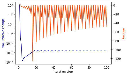
Even though the pole relocation process oscillated between two (or more?) solutions and did not converge, the fit was still successful, because the solutions themselves did converge:

vf.get_rms_error()

0.0278797454068358

fig, ax = mplt.subplots(2, 2)
fig.set_size_inches(12, 8)
vf.plot_s_mag(0, 0, freqs=freqs, ax=ax[0][0]) # s11
vf.plot_s_mag(0, 1, freqs=freqs, ax=ax[0][1]) # s12
vf.plot_s_mag(1, 0, freqs=freqs, ax=ax[1][0]) # s21
vf.plot_s_mag(1, 1, freqs=freqs, ax=ax[1][1]) # s22
fig.tight_layout()
mplt.show()