Download This Notebook: Media.ipynb

Media

Introduction

skrf supports some basic circuit simulation based on transmission line models. Network creation is accomplished through methods of the Media class, which represents a transmission line object for a given medium. Once constructed, a Media object contains the necessary properties such as propagation constant and characteristic impedance, that are needed to generate microwave networks.

This tutorial illustrates how created Networks using several different Media objects. The basic usage is,

%matplotlib inline
import skrf as rf
rf.stylely()

from skrf import Frequency
from skrf.media import CPW

freq = Frequency(75,110,101,'ghz')
cpw =  CPW(freq, w=10e-6, s=5e-6, ep_r=10.6)
cpw

Coplanar Waveguide Media.  75-110 GHz.  101 points
 W= 1.00e-05m, S= 5.00e-06m

To create a transmission line of 100um

cpw.line(100*1e-6, name = '100um line')

2-Port Network: '100um line',  75.0-110.0 GHz, 101 pts, z0=[50.0283242+0.j 50.0283242+0.j]

More detailed examples illustrating how to create various kinds of Media objects are given below. A full list of media’s supported can be found in the Media API page. The network creation and connection syntax of skrf are cumbersome if you need to doing complex circuit design. skrf’s synthesis capabilities lend themselves more to scripted applications such as calibration, optimization or batch processing.

Media Object Basics

Two arguments are common to all media constructors

• frequency (required)

• z0 (optional)

frequency is a Frequency object, and z0 is the port impedance. z0 is only needed if the port impedance is different from the media’s characteristic impedance. Here is an example of how to initialize a coplanar waveguide [0] media. The instance has a 10um center conductor, gap of 5um, and substrate with relative permativity of 10.6,

freq = Frequency(75,110,101,'ghz')
cpw = CPW(freq, w=10e-6, s=5e-6, ep_r=10.6, z0 =1)

cpw

Coplanar Waveguide Media.  75-110 GHz.  101 points
 W= 1.00e-05m, S= 5.00e-06m

For the purpose of microwave network analysis, the defining properties of a (single moded) transmission line are it’s characteristic impedance and propagation constant. These properties return complex numpy.ndarray’s, A port impedance is also needed when different networks are connected.

The characteristic impedance is given by a Z0 (capital Z)

cpw.Z0[:3]

array([50.0283242+0.j, 50.0283242+0.j, 50.0283242+0.j])

The port impedance is given by z0 (lower z). Which we set to 1, just to illustrate how this works. The port impedance is used to compute impedance mismatched if circuits of different port impedance are connected.

cpw.z0[:3]

array([1., 1., 1.])

The propagation constant is given by gamma

cpw.gamma[:3]

array([0.+3785.59740814j, 0.+3803.26352937j, 0.+3820.92965061j])

Lets take a look at some other Media’s

Slab of Si in Freespace

A plane-wave in freespace from 10-20GHz.

from skrf.media import Freespace

freq = Frequency(10,20,101,'ghz')
air =  Freespace(freq)
air

Freespace  Media.  10-20 GHz.  101 points

air.z0[:2] # 377ohm baby!

array([376.73031367+0.j, 376.73031367+0.j])

# plane wave in Si
si = Freespace(freq, ep_r = 11.2)
si.z0[:3] # ~110ohm

array([112.56971222+0.j, 112.56971222+0.j, 112.56971222+0.j])

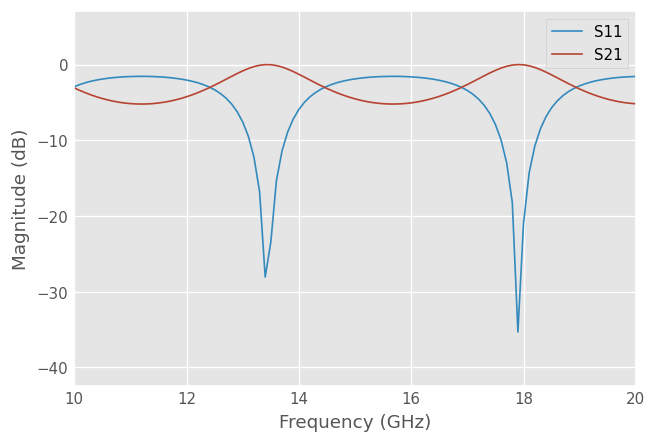
Simulate a 1cm slab of Si in half-space,

slab = air.thru() ** si.line(1, 'cm') ** air.thru()
slab.plot_s_db(n=0)

Rectangular Waveguide

a WR-10 Rectangular Waveguide

from skrf.media import RectangularWaveguide

freq = Frequency(75,110,101,'ghz')
wg = RectangularWaveguide(freq, a=100*rf.mil, z0=50) # see note below about z0
wg

Rectangular Waveguide Media.  75-110 GHz.  101 points
 a= 2.54e-03m, b= 1.27e-03m

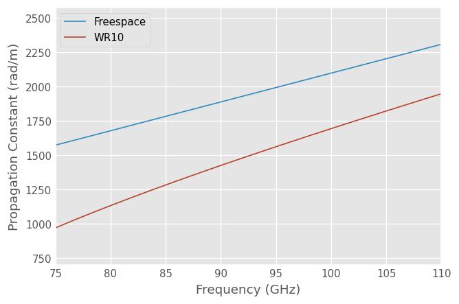
The z0 argument in the Rectangular Waveguide constructor is used to force a specific port impedance. This is commonly used to match the port impedance to what a VNA stores in a touchstone file. Lets compare the propagation constant in waveguide to that of freespace,

air = Freespace(freq)

from matplotlib import pyplot as plt

air.plot(air.gamma.imag, label='Freespace')
wg.plot(wg.gamma.imag, label='WR10')

plt.ylabel('Propagation Constant (rad/m)')
plt.legend()

<matplotlib.legend.Legend at 0x7f018efbcd00>

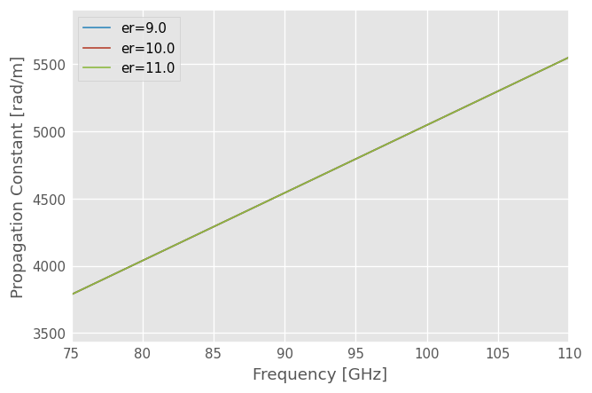
Because the wave quantities are dynamic they change when the attributes of the media change. To illustrate, plot the propagation constant of the cpw for various values of substrated permativity,

for ep_r in [9,10,11]:
    cpw.ep_r = ep_r
    cpw.frequency.plot(cpw.beta, label='er=%.1f'%ep_r)

plt.xlabel('Frequency [GHz]')
plt.ylabel('Propagation Constant [rad/m]')
plt.legend()

<matplotlib.legend.Legend at 0x7f018ef4b8b0>

Network Synthesis

Networks are created through methods of a Media object. To create a 1-port network for a rectangular waveguide short,

wg.short(name = 'short')

1-Port Network: 'short',  75.0-110.0 GHz, 101 pts, z0=[50.+0.j]

Or to create a \(90^{\circ}\) section of cpw line,

cpw.line(d=90,unit='deg', name='line')

2-Port Network: 'line',  75.0-110.0 GHz, 101 pts, z0=[1.+0.j 1.+0.j]

Note

Simple circuits like :Media.short and open are ideal short and opens with $Gamma = -1$ and $Gamma = 1$, i.e. they dont take into account sophisticated effects of the discontinuities. Eventually, these more complex networks could be implemented with

methods specific to a given Media, ie CPW.cpw_short , should the need arise…

Building Circuits

By connecting a series of simple circuits, more complex circuits can be made. To build a the \(90^{\circ}\) delay short, in the rectangular waveguide media defined above.

delay_short = wg.line(d=90,unit='deg') ** wg.short()
delay_short.name = 'delay short'
delay_short

1-Port Network: 'delay short',  75.0-110.0 GHz, 101 pts, z0=[50.+0.j]

When Networks with more than 2 ports need to be connected together, use rf.connect(). To create a two-port network for a shunted delayed open, you can create an ideal 3-way splitter (a ‘tee’) and connect the delayed open to one of its ports,

tee = cpw.tee()
delay_open = cpw.delay_open(40,'deg')
shunt_open = rf.connect(tee,1,delay_open,0)

Adding networks in shunt is pretty common, so there is a Media.shunt() function to do this,

cpw.shunt(delay_open)

2-Port Network: '',  75.0-110.0 GHz, 101 pts, z0=[1.+0.j 1.+0.j]

If a specific circuit is created frequently, it may make sense to use a function to create the circuit. This can be done most quickly using lambda

delay_short = lambda d: wg.line(d,'deg')**wg.short()
delay_short(90)

1-Port Network: '',  75.0-110.0 GHz, 101 pts, z0=[50.+0.j]

A more useful example may be to create a function for a shunt-stub tuner, that will work for any media object

def shunt_stub(med, d0, d1):
    return med.line(d0,'deg')**med.shunt_delay_open(d1,'deg')

shunt_stub(cpw,10,90)

2-Port Network: '',  75.0-110.0 GHz, 101 pts, z0=[1.+0.j 1.+0.j]

This approach lends itself to design optimization.

Design Optimization

The abilities of scipy‘s optimizers can be used to automate network design. In this example, skrf is used to automate the single stub impedance matching network design. First, we create a ’cost’ function which returns something we want to minimize, such as the reflection coefficient magnitude at band center. Then, one of scipy’s minimization algorithms is used to determine the optimal parameters of the stub lengths to minimize this cost.

from scipy.optimize import fmin

# the load we are trying to match
load = cpw.load(.2+.2j)

# single stub circuit generator function
def shunt_stub(med, d0, d1):
    return med.line(d0,'deg')**med.shunt_delay_open(d1,'deg')


# define the cost function we want to minimize (this uses sloppy namespace)
def cost(d):
    # prevent negative length lines, returning high cost
    if d[0] <0 or d[1] <0:
        return 1e3
    return (shunt_stub(cpw,d[0],d[1]) ** load)[100].s_mag.squeeze()

# initial guess of optimal delay lengths in degrees
d0 = 120,40 # initial guess

#determine the optimal delays
d_opt = fmin(cost,(120,40))

d_opt

Optimization terminated successfully.
         Current function value: 0.233333
         Iterations: 58
         Function evaluations: 125

array([174.64452415,  12.71791558])