Download This Notebook: Networks.ipynb
Networks
Introduction
This tutorial gives an overview of the microwave network analysis features of skrf. For this tutorial, and the rest of the scikit-rf documentation, it is assumed that skrf has been imported as rf. Whether or not you follow this convention in your own code is up to you.
[1]:
import skrf as rf
from pylab import *
If this produces an import error, please see Installation.
Creating Networks
skrf provides an object for a N-port microwave Network. A Network can be created in a number of ways: - from a Touchstone file - from S-parameters - from Z-parameters - from other RF parameters (Y, ABCD, T, etc.)
Some examples for each situation is given below.
Creating Network from Touchstone file
Touchstone file (.sNp files, with N being the number of ports) is a de facto standard to export N-port network parameter data and noise data of linear active devices, passive filters, passive devices, or interconnect networks. Creating a Network from a Touchstone file is simple:
[2]:
from skrf import Network, Frequency

ring_slot = Network('data/ring slot.s2p')
Note that some softwares, such as ANSYS HFSS, add additional information to the Touchstone standard, such as comments, simulation parameters, Port Impedance or Gamma (wavenumber). These data are also imported if detected.
A short description of the network will be printed out if entered onto the command line
[3]:
ring_slot
[3]:
2-Port Network: 'ring slot', 75.0-110.0 GHz, 201 pts, z0=[50.+0.j 50.+0.j]
Creating Network from s-parameters
Networks can also be created by directly passing values for the frequency, s-parameters (and optionally the port impedance z0).
The scattering matrix of a N-port Network is expected to be a Numpy array of shape (nb_f, N, N), where nb_f is the number of frequency points and N the number of ports of the network.

[4]:
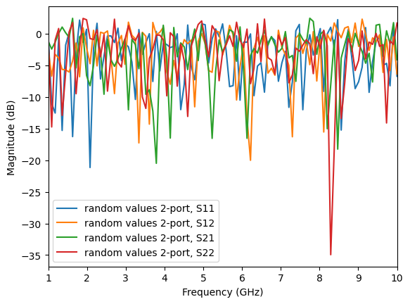
# dummy 2-port network from Frequency and s-parameters
freq = Frequency(1, 10, 101, 'ghz')
s = rand(101, 2, 2) + 1j*rand(101, 2, 2)  # random complex numbers
# if not passed, will assume z0=50. name is optional but it's a good practice.
ntwk = Network(frequency=freq, s=s, name='random values 2-port')
ntwk
[4]:
2-Port Network: 'random values 2-port', 1.0-10.0 GHz, 101 pts, z0=[50.+0.j 50.+0.j]
[5]:
ntwk.plot_s_db()
Often, s-parameters are stored in separate arrays. In such case, one needs to forge the s-matrix:
[6]:
# let's assume we have separate arrays for the frequency and s-parameters
f = np.array([1, 2, 3, 4]) # in GHz
S11 = np.random.rand(4)
S12 = np.random.rand(4)
S21 = np.random.rand(4)
S22 = np.random.rand(4)

# Before creating the scikit-rf Network object, one must forge the Frequency and S-matrix:
freq2 = rf.Frequency.from_f(f, unit='GHz')

# forging S-matrix as shape (nb_f, 2, 2)
# there is probably smarter way, but less explicit for the purpose of this example:
s = np.zeros((len(f), 2, 2), dtype=complex)
s[:,0,0] = S11
s[:,0,1] = S12
s[:,1,0] = S21
s[:,1,1] = S22

# constructing Network object
ntw = rf.Network(frequency=freq2, s=s)

print(ntw)
2-Port Network: '', 1.0-4.0 GHz, 4 pts, z0=[50.+0.j 50.+0.j]
If necessary, the characteristic impedance can be passed as a scalar (same for all frequencies), as a list or an array:
[7]:
ntw2 = rf.Network(frequency=freq, s=s, z0=25, name='same z0 for all ports')
print(ntw2)
ntw3 = rf.Network(frequency=freq, s=s, z0=[20, 30], name='different z0 for each port')
print(ntw3)
ntw4 = rf.Network(frequency=freq, s=s, z0=rand(4,2), name='different z0 for each frequencies and ports')
print(ntw4)
2-Port Network: 'same z0 for all ports',  1.0-10.0 GHz, 101 pts, z0=[25.+0.j 25.+0.j]
2-Port Network: 'different z0 for each port',  1.0-10.0 GHz, 101 pts, z0=[20.+0.j 30.+0.j]
2-Port Network: 'different z0 for each frequencies and ports',  1.0-10.0 GHz, 101 pts, z0=[0.38605005+0.j 0.14804491+0.j]
From z-parameters
As networks are also defined from their Z-parameters, there is from_z() method of the Network:
[8]:
# 1-port network example
z = np.full((len(freq), 1, 1), 10j)  # replicate z=10j for all frequencies

ntw = rf.Network(frequency=freq, z=z)
print(ntw)
1-Port Network: '', 1.0-10.0 GHz, 101 pts, z0=[50.+0.j]
From other network parameters: Y, ABCD, H, T
It is also possible to generate Networks from other kind of RF parameters: Y, ABCD, H or T using the y=, a=, h= or t= parameters
respectively when creating a Network.
For example, the ABCD parameters of a series-impedance is:
so the associated Network can be created like:
[9]:
z = 20
abcd = array([[1, z],
              [0, 1]])

a = tile(abcd, (len(freq),1,1))
ntw = Network(frequency=freq, a=a)
print(ntw)
2-Port Network: '', 1.0-10.0 GHz, 101 pts, z0=[50.+0.j 50.+0.j]
Note that convenience functions are also available for converting some parameters into another if required:
from:nbsphinx-math:to |
S |
Z |
Y |
ABCD |
T |
H |
|---|---|---|---|---|---|---|
S |
|
|
|
|
|
|
Z |
|
|
|
|
|
|
Y |
|
|
|
|||
ABCD |
|
|
||||
T |
|
|
|
|||
H |
|
|
[10]:
# example: converting a -> s
s = rf.a2s(a)
# checking that these S-params are the same
np.all(ntw.s == s)
[10]:
True
Basic Properties
The basic attributes of a microwave Network are provided by the following properties :
Network.s: Scattering Parameter matrix.Network.z0: Port Characteristic Impedance matrix.Network.frequency: Frequency Object.
The Network object has numerous other properties and methods. If you are using IPython, then these properties and methods can be ‘tabbed’ out on the command line.
In [1]: ring_slot.s<TAB>
ring_slot.line.s              ring_slot.s_arcl         ring_slot.s_im
ring_slot.line.s11            ring_slot.s_arcl_unwrap  ring_slot.s_mag
...
All of the network parameters are represented internally as complex numpy.ndarray. The s-parameters are of shape (nfreq, nport, nport):
[11]:
shape(ring_slot.s)
[11]:
(201, 2, 2)
Slicing
You can slice the Network.s attribute any way you want.
[12]:
ring_slot.s[:11,1,0] # get first 10 values of S21
[12]:
array([0.6134571 +0.36678139j, 0.6218194 +0.36403169j,
       0.63024301+0.36109574j, 0.63872415+0.3579682j ,
       0.64725874+0.35464377j, 0.65584238+0.35111711j,
       0.66447037+0.34738295j, 0.6731377 +0.34343602j,
       0.68183901+0.33927115j, 0.69056862+0.33488321j,
       0.6993205 +0.3302672j ])
Slicing by frequency can also be done directly on Network objects like so
[13]:
ring_slot[0:10] # Network for the first 10 frequency points
[13]:
2-Port Network: 'ring slot_subset', 75.0-76.575 GHz, 10 pts, z0=[50.+0.j 50.+0.j]
or with a human friendly string,
[14]:
ring_slot['80-90ghz']
[14]:
2-Port Network: 'ring slot', 80.075-90.05 GHz, 58 pts, z0=[50.+0.j 50.+0.j]
Notice that slicing directly on a Network returns a Network. So, a nice way to express slicing in both dimensions is
[15]:
ring_slot.s11['80-90ghz']
[15]:
1-Port Network: 'ring slot', 80.075-90.05 GHz, 58 pts, z0=[50.+0.j]
Plotting
Amongst other things, the methods of the Network class provide convenient ways to plot components of the network parameters,
Network.plot_s_db: plot magnitude of s-parameters in log scaleNetwork.plot_s_deg: plot phase of s-parameters in degreesNetwork.plot_s_smith: plot complex s-parameters on Smith Chart…
If you would like to use skrf’s plot styling,
[16]:
%matplotlib inline
rf.stylely()
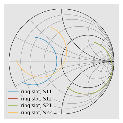
To plot all four s-parameters of the ring_slot on the Smith Chart.
[17]:
ring_slot.plot_s_smith()
Combining this with the slicing features,
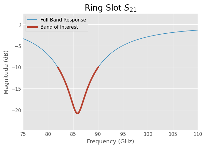
[18]:
from matplotlib import pyplot as plt

plt.title('Ring Slot $S_{21}$')

ring_slot.s11.plot_s_db(label='Full Band Response')
ring_slot.s11['82-90ghz'].plot_s_db(lw=3,label='Band of Interest')
For more detailed information about plotting see Plotting.
Arithmetic Operations
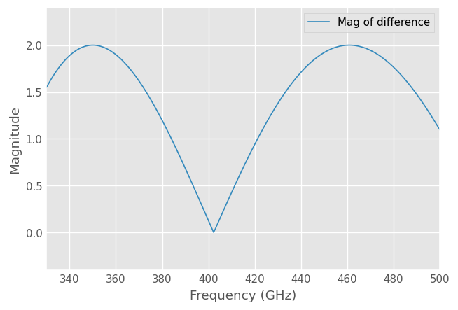
Element-wise mathematical operations on the scattering parameter matrices are accessible through overloaded operators. To illustrate their usage, load a couple Networks stored in the data module.
[19]:
from skrf.data import wr2p2_short as short
from skrf.data import wr2p2_delayshort as delayshort


short - delayshort
short + delayshort
short * delayshort
short / delayshort
[19]:
1-Port Network: 'wr2p2,short', 330.0-500.0 GHz, 201 pts, z0=[50.+0.j]
All of these operations return Network types. For example, to plot the complex difference between short and delay_short,
[20]:
difference = (short - delayshort)
difference.plot_s_mag(label='Mag of difference')
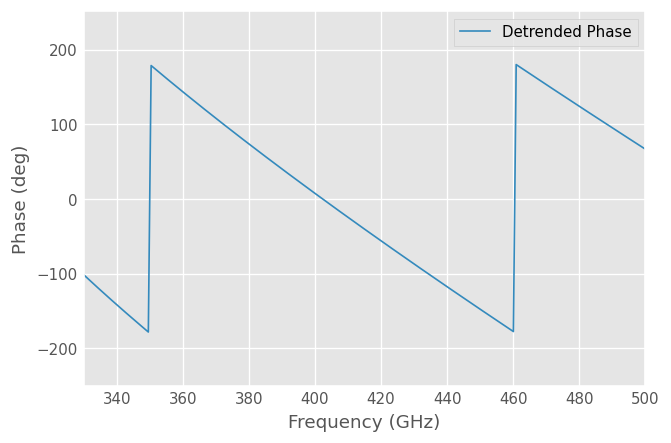
Another common application is calculating the phase difference using the division operator,
[21]:
(delayshort/short).plot_s_deg(label='Detrended Phase')
Linear operators can also be used with scalars or an numpy.ndarray that ais the same length as the Network.
[22]:
hopen = (short*-1)
hopen.s[:3,...]
[22]:
array([[[1.-0.j]],

       [[1.-0.j]],

       [[1.-0.j]]])
[23]:
rando =  hopen *rand(len(hopen))
rando.s[:3,...]
[23]:
array([[[0.61875425+0.j]],

       [[0.51928795+0.j]],

       [[0.33892295+0.j]]])
Comparison of Network
Comparison operators also work with networks:
[24]:
short == delayshort
[24]:
False
[25]:
short != delayshort
[25]:
True
Cascading and De-embedding
Cascading and de-embeding 2-port Networks can also be done through operators. The cascade function can be called through the power operator, **. To calculate a new network which is the cascaded connection of the two individual Networks line and short,
[26]:
short = rf.data.wr2p2_short
line = rf.data.wr2p2_line
delayshort = line ** short
De-embedding can be accomplished by cascading the inverse of a network. The inverse of a network is accessed through the property Network.inv. To de-embed the short from delay_short,
[27]:
short_2 = line.inv ** delayshort

short_2 == short
[27]:
True
The cascading operator also works for to 2N-port Networks. This is illustrated in this example on balanced Networks. For example, assuming you want to cascade three 4-port Network ntw1, ntw2 and ntw3, you can use: resulting_ntw = ntw1 ** ntw2 ** ntw3. Note that the port scheme assumed by the ** cascading operator with 4-port networks is:
   ntw1    ntw2    ntw3
  +----+  +----+  +----+
0-|0  2|--|0  2|--|0  2|-2
1-|1  3|--|1  3|--|1  3|-3
  +----+  +----+  +----+
More documentation on Connecting Network is available here: Connecting Networks.
Connecting Multi-ports
skrf supports the connection of arbitrary ports of N-port networks. It accomplishes this using an algorithm called sub-network growth[1], available through the function connect().
As an example, terminating one port of an ideal 3-way splitter can be done like so,
[28]:
tee = rf.data.tee
tee
[28]:
3-Port Network: 'tee', 330.0-500.0 GHz, 201 pts, z0=[50.+0.j 50.+0.j 50.+0.j]
To connect port 1 of the tee, to port 0 of the delay short,
[29]:
terminated_tee = rf.connect(tee, 1, delayshort, 0)
terminated_tee
[29]:
2-Port Network: 'tee', 330.0-500.0 GHz, 201 pts, z0=[50.+0.j 50.+0.j]
Note that this function takes into account port impedances. If two connected ports have different port impedances, an appropriate impedance mismatch is inserted.
More information on connecting Networks is available here: connecting Networks.
For advanced connections between many arbitrary N-port Networks, the Circuit object is more relevant since it allows defining explicitly the connections between ports and Networks. For more information, please refer to the Circuit documentation.
Interpolation and Concatenation
A common need is to change the number of frequency points of a Network. To use the operators and cascading functions the networks involved must have matching frequencies, for instance. If two networks have different frequency information, then an error will be raised,
[30]:
from skrf.data import wr2p2_line1 as line1

line1
[30]:
2-Port Network: 'wr2p2,line1', 330.0-500.0 GHz, 101 pts, z0=[50.+0.j 50.+0.j]
line1+line

---------------------------------------------------------------------------
IndexError                                Traceback (most recent call last)
<ipython-input-49-82040f7eab08> in <module>()
----> 1 line1+line

/home/alex/code/scikit-rf/skrf/network.py in __add__(self, other)
    500
    501         if isinstance(other, Network):
--> 502             self.__compatible_for_scalar_operation_test(other)
    503             result.s = self.s + other.s
    504         else:

/home/alex/code/scikit-rf/skrf/network.py in __compatible_for_scalar_operation_test(self, other)
    701         '''
    702         if other.frequency  != self.frequency:
--> 703             raise IndexError('Networks must have same frequency. See `Network.interpolate`')
    704
    705         if other.s.shape != self.s.shape:

IndexError: Networks must have same frequency. See `Network.interpolate`
This problem can be solved by interpolating one of Networks along the frequency axis using Network.resample.
[31]:
line1.resample(201)
line1
[31]:
2-Port Network: 'wr2p2,line1', 330.0-500.0 GHz, 201 pts, z0=[50.+0.j 50.+0.j]
And now we can do things
[32]:
line1 + line
[32]:
2-Port Network: 'wr2p2,line1', 330.0-500.0 GHz, 201 pts, z0=[50.+0.j 50.+0.j]
You can also interpolate from a Frequency object. For example,
[33]:
line.interpolate(line1.frequency)
[33]:
2-Port Network: 'wr2p2,line', 330.0-500.0 GHz, 201 pts, z0=[50.+0.j 50.+0.j]
A related application is the need to combine Networks which cover different frequency ranges. Two Networks can be concatenated (aka stitched) together using stitch, which concatenates networks along their frequency axis. To combine a WR-2.2 Network with a WR-1.5 Network,
[34]:
from skrf.data import wr2p2_line, wr1p5_line

big_line = rf.stitch(wr2p2_line, wr1p5_line)
big_line
/home/docs/checkouts/readthedocs.org/user_builds/scikit-rf/envs/v0.24.0/lib/python3.10/site-packages/skrf/frequency.py:324: InvalidFrequencyWarning: Frequency values are not monotonously increasing!
To get rid of the invalid values call `drop_non_monotonic_increasing`
  warnings.warn("Frequency values are not monotonously increasing!\n"
[34]:
2-Port Network: 'wr2p2,line', 330.0-750.0 GHz, 402 pts, z0=[50.+0.j 50.+0.j]
Reading and Writing
For long term data storage, skrf has support for reading and partial support for writing touchstone file format. Reading is accomplished with the Network initializer as shown above, and writing with the method Network.write_touchstone().
For temporary data storage, skrf object can be pickled with the functions skrf.io.general.read and skrf.io.general.write. The reason to use temporary pickles over touchstones is that they store all attributes of a network, while touchstone files only store partial information.
[35]:
rf.write('data/myline.ntwk',line) # write out Network using pickle
[36]:
ntwk = Network('data/myline.ntwk') # read Network using pickle
Warning
Pickling methods cant support long term data storage because they require the structure of the object being written to remain unchanged. something that cannot be guaranteed in future versions of skrf. (see http://docs.python.org/2/library/pickle.html)
Frequently there is an entire directory of files that need to be analyzed. rf.read_all creates Networks from all files in a directory quickly. To load all skrf files in the data/ directory which contain the string 'wr2p2'.
[37]:
dict_o_ntwks = rf.read_all(rf.data.pwd, contains = 'wr2p2')
dict_o_ntwks
[37]:
{'wr2p2,delayshort': 1-Port Network: 'wr2p2,delayshort',  330.0-500.0 GHz, 201 pts, z0=[50.+0.j],
 'wr2p2,line': 2-Port Network: 'wr2p2,line',  330.0-500.0 GHz, 201 pts, z0=[50.+0.j 50.+0.j],
 'wr2p2,line1': 2-Port Network: 'wr2p2,line1',  330.0-500.0 GHz, 101 pts, z0=[50.+0.j 50.+0.j],
 'wr2p2,short': 1-Port Network: 'wr2p2,short',  330.0-500.0 GHz, 201 pts, z0=[50.+0.j]}
Other times you know the list of files that need to be analyzed. rf.read_all also accepts a files parameter. This example file list contains only files within the same directory, but you can store files however your application would benefit from.
[38]:
import os
dict_o_ntwks_files = rf.read_all(files=[os.path.join(rf.data.pwd, test_file) for test_file in ['ntwk1.s2p', 'ntwk2.s2p']])
dict_o_ntwks_files
[38]:
{'ntwk1': 2-Port Network: 'ntwk1', 1.0-10.0 GHz, 91 pts, z0=[50.+0.j 50.+0.j]}
Other Parameters
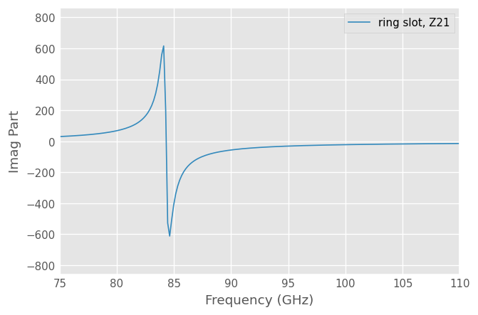
This tutorial focuses on s-parameters, but other network representations are available as well. Impedance and Admittance Parameters can be accessed through the parameters Network.z and Network.y, respectively. Scalar components of complex parameters, such as Network.z_re, Network.z_im and plotting methods are available as well.
Other parameters are only available for 2-port networks, such as wave cascading parameters (Network.t), and ABCD-parameters (Network.a) or Hybrid parameters (Network.h).
[39]:
ring_slot.z[:3,...]
[39]:
array([[[0.88442687+28.15350224j, 0.94703504+30.46757222j],
        [0.94703504+30.46757222j, 1.0434417 +43.45766805j]],

       [[0.91624901+28.72415928j, 0.98188607+31.09594438j],
        [0.98188607+31.09594438j, 1.08168411+44.17642274j]],

       [[0.94991736+29.31694632j, 1.01876516+31.74874257j],
        [1.01876516+31.74874257j, 1.12215451+44.92215712j]]])
[40]:
ring_slot.plot_z_im(m=1,n=0)
References
[1] Compton, R.C.; , “Perspectives in microwave circuit analysis,” Circuits and Systems, 1989., Proceedings of the 32nd Midwest Symposium on , vol., no., pp.716-718 vol.2, 14-16 Aug 1989. URL: http://ieeexplore.ieee.org/stamp/stamp.jsp?tp=&arnumber=101955&isnumber=3167
[ ]: