Properties of Rectangular Waveguide
Introduction
This example demonstrates how to use scikit-rf to calculate some properties of rectangular waveguide. For more information regarding the theoretical basis for these calculations, see the References.
Object Creation
This first section imports necessary modules and creates several RectangularWaveguide objects for some standard waveguide bands.
[1]:
%matplotlib inline
# imports
import matplotlib.pyplot as plt
import numpy as np
from scipy.constants import c, mil

import skrf as rf
from skrf.frequency import Frequency
from skrf.mathFunctions import np_2_db
from skrf.media import Freespace, RectangularWaveguide

rf.stylely()
# plot formatting
plt.rcParams['lines.linewidth'] = 2
[2]:
# create frequency objects for standard bands
f_wr5p1  = Frequency(140,220,1001, 'GHz')
f_wr3p4  = Frequency(220,330,1001, 'GHz')
f_wr2p2 = Frequency(330,500,1001, 'GHz')
f_wr1p5 = Frequency(500,750,1001, 'GHz')
f_wr1   = Frequency(750,1100,1001, 'GHz')

# create rectangular waveguide objects
wr5p1 = RectangularWaveguide(f_wr5p1.copy(), a=51*mil, b=25.5*mil, rho = 'au')
wr3p4 = RectangularWaveguide(f_wr3p4.copy(), a=34*mil, b=17*mil, rho = 'au')
wr2p2 = RectangularWaveguide(f_wr2p2.copy(), a=22*mil, b=11*mil, rho = 'au')
wr1p5 = RectangularWaveguide(f_wr1p5.copy(), a=15*mil, b=7.5*mil, rho = 'au')
wr1   = RectangularWaveguide(f_wr1.copy(), a=10*mil, b=5*mil, rho = 'au')

# add names to waveguide objects for use in plot legends
wr5p1.name = 'WR-5.1'
wr3p4.name = 'WR-3.4'
wr2p2.name = 'WR-2.2'
wr1p5.name = 'WR-1.5'
wr1.name = 'WR-1.0'

# create a list to iterate through
wg_list = [wr5p1, wr3p4,wr2p2,wr1p5,wr1]

# creat a freespace object too
freespace = Freespace(Frequency(125,1100, 1001, 'GHz'))
freespace.name = 'Free Space'
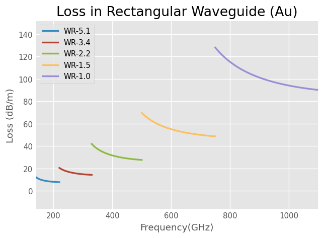
Conductor Loss
[3]:
fig, ax = plt.subplots()

for wg in wg_list:
    wg.frequency.plot(np_2_db(wg.alpha), label=wg.name)

ax.legend()
ax.set_xlabel('Frequency(GHz)')
ax.set_ylabel('Loss (dB/m)')
ax.set_title('Loss in Rectangular Waveguide (Au)');
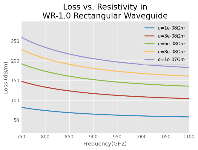
[4]:
fig, ax = plt.subplots()
resistivity_list = np.linspace(1,10,5)*1e-8 # ohm meter
for rho in resistivity_list:
    wg = RectangularWaveguide(f_wr1.copy(), a=10*mil, b=5*mil,
                              rho = rho)
    wg.frequency.plot(np_2_db(wg.alpha),label=rf'$ \rho $={rho:e}$ \Omega m$')

ax.legend()
ax.set_xlabel('Frequency(GHz)')
ax.set_ylabel('Loss (dB/m)')
ax.set_title('Loss vs. Resistivity in\nWR-1.0 Rectangular Waveguide');
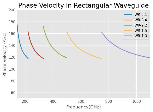
Phase and Group Velocity
[5]:
fig, ax = plt.subplots()
for wg in wg_list:
    wg.frequency.plot(100*wg.v_p.real/c, label=wg.name )

ax.legend()
ax.set_ylim(50,200)
ax.set_xlabel('Frequency(GHz)')
ax.set_ylabel(r'Phase Velocity (\%c)')
ax.set_title('Phase Velocity in Rectangular Waveguide');
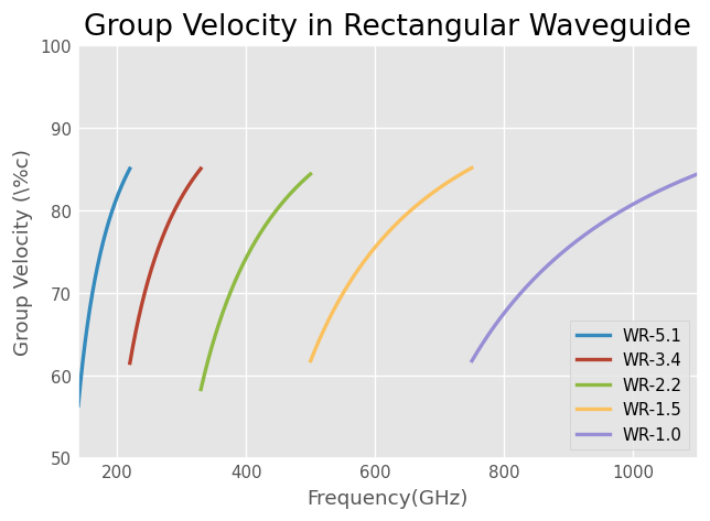
[6]:
fig, ax = plt.subplots()
for wg in wg_list:
    plt.plot(wg.frequency.f_scaled[1:],
             100/c*np.diff(wg.frequency.w)/np.diff(wg.beta),
             label=wg.name )

ax.legend()
ax.set_ylim(50,100)
ax.set_xlabel('Frequency(GHz)')
ax.set_ylabel(r'Group Velocity (\%c)')
ax.set_title('Group Velocity in Rectangular Waveguide');
Propagation Constant
[7]:
fig, ax = plt.subplots()
for wg in wg_list+[freespace]:
    wg.frequency.plot(wg.beta,   label=wg.name)

ax.legend()
ax.set_xlabel('Frequency(GHz)')
ax.set_ylabel('Propagation Constant (rad/m)')
ax.set_title('Propagation Constant \nin Rectangular Waveguide')
ax.semilogy()
[7]:
[]

References
[1] https://www.microwaves101.com/encyclopedias/waveguide-mathematics
[2] http://en.wikipedia.org/wiki/Waveguide_(electromagnetism)
[3] R. F. Harrington, Time-Harmonic Electromagnetic Fields (IEEE Press Series on Electromagnetic Wave Theory). Wiley-IEEE Press, 2001.
[4] http://www.ece.rutgers.edu/~orfanidi/ewa (see Chapter 9)