Renormalizing S-parameters

This example demonstrates how to use skrf to renormalize a Network’s s-parameters to new port impedances. Although trivial, this example creates a matched load in 50ohms and then re-normalizes to a 25ohm environment, producing a reflection coefficient of 1/3.

Ok lets do it

import skrf as rf
%matplotlib inline
from pylab import *
rf.stylely()

# this is just for plotting junk
kw = dict(draw_labels=True, marker = 'o', markersize = 10)

Create a one-port ideal match Network, (using the premade media class wr10 as a dummy)

match_at_50 = rf.wr10.match()

Note that the z0 for this Network defaults to a constant 50ohm

match_at_50

1-Port Network: '',  75.0-110.0 GHz, 1001 pts, z0=[50.+0.j]

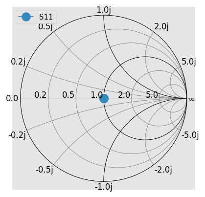
Plotting its reflection coefficient on the smith chart, shows its a match

match_at_50.plot_s_smith(**kw)

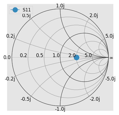
Now, renormalize the port impedance from 50 -> 25, thus the previous 50ohm load now produces a reflection coefficient of

\[\Gamma^{'} = \frac{50-25}{50+25} = \frac{25}{75} = .333\]

Plotting the renormalized response on the Smith Chart

match_at_50.renormalize(25)
match_at_50.plot_s_smith(**kw)

Complex Impedances

You could also renormalize to a complex port impedance if you’re crazy. For example, renormalizing to 50j, one would expect:

\[\Gamma^{'} = \frac{50-50j}{50+50j} = 50\frac{1-j}{1+j} = -50j\]

However, one finds an unexpected result when plotting the Smith chart:

match_at_50 = rf.wr10.match()
match_at_50.renormalize(50j)  # same as renormalize(50j, s_def='power')
match_at_50.plot_s_smith(**kw)  # expect -1j

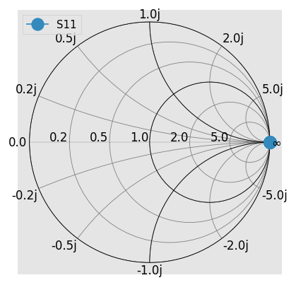
This is because the default behaviour of scikit-rf is to use power-waves scattering parameter definition (since it is the most popular one is CAD softwares). But the power-waves definition is known to fail in such a case. This is why scikit-rf also implement the pseudo-waves scattering parameters definition, but you have to specify it using the s_def parameter:

match_at_50 = rf.wr10.match()
match_at_50.renormalize(50j, s_def='pseudo')
match_at_50.plot_s_smith(**kw)  # expect -1j

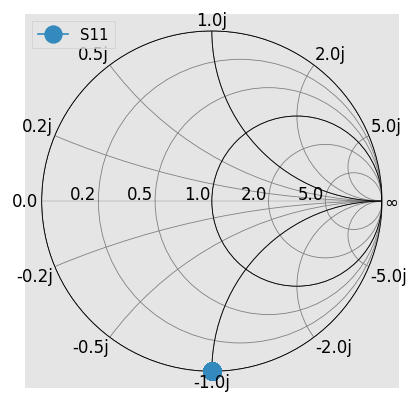
Which gives the expected result.