Modeling Transmission Line Properties

Table of Contents

• Introduction

• Propagation constant

• Interlude on attenuation units

• Modeling a loaded lossy transmission line using transmission line functions

• Input impedances, reflection coefficients and SWR

• Voltages and Currents

• Modeling a loaded lossy transmission line by cascading Networks

• Determination of the propagation constant from the input impedance

Introduction

In this tutorial, scikit-rf is used to work with some classical transmission line situations, such as calculating impedances, reflection coefficients, standing wave ratios or voltages and currents. There is at least two way of performing these calculations, one using transmission line functions or by creating and cascading Networks

Let’s consider a lossy coaxial cable of characteristic impedance \(Z_0=75 \Omega\) of length \(d=12 m\). The coaxial cable has an attenuation of 0.02 Neper/m and a velocity factor VF=0.67 (This corresponds roughly to a RG-6 coaxial). The cable is loaded with a \(Z_L=150 \Omega\) impedance. The RF frequency of interest is 250 MHz.

Please note that in scikit-rf, the line length is defined from the load, ie \(z=0\) at the load and \(z=d\) at the input of the transmission line:

First, let’s make the necessary Python import statements:

%matplotlib inline
import skrf as rf
from pylab import *

# skrf figure styling
rf.stylely()

And the constants of the problem:

freq = rf.Frequency(250, npoints=1, unit='MHz')
Z_0 = 75  # Ohm
Z_L = 150  # Ohm
d = 12  # m
VF = 0.67
att = 0.02 # Np/m. Equivalent to 0.1737 dB/m

Before going into impedance and reflection coefficient calculations, first we need to define the transmission line properties, in particular its propagation constant.

Propagation constant

In order to get the RF parameters of the transmission line, it is necessary to derive the propagation constant of the line. The propagation constant \(\gamma\) of the line is defined in scikit-rf as \(\gamma=\alpha + j\beta\) where \(\alpha\) is the attenuation (in Neper/m) and \(\beta=\frac{2\pi}{\lambda}=\frac{\omega}{c}/\mathrm{VF}=\frac{\omega}{c}\sqrt{\epsilon_r}\) the phase constant.

First, the wavelength in the coaxial cable is

\[\lambda=\frac{c}{f \sqrt{\epsilon_r}}=\frac{c}{f} \mathrm{VF}\]

lambd = rf.c/freq.f * VF
print('VF=', VF, 'and Wavelength:', lambd, 'm')

VF= 0.67 and Wavelength: [0.80344379] m

As the attenuation is already given in Np/m, the propagation constant is:

alpha = att  # Np/m !
beta = freq.w/rf.c/VF
gamma = alpha + 1j*beta
print('Transmission line propagation constant: gamma = ', gamma, 'rad/m')

Transmission line propagation constant: gamma =  [0.02+7.82031725j] rad/m

If the attenuation would have been given in other units, scikit-rf provides the necessary tools to convert units, as described below.

Interlude: On Attenuation Units

Attenuation is generally provided (or expected) in various kind of units. scikit-rf provides convenience functions to manipulate line attenuation units.

For example, the cable attenuation given in Np/m, can be expressed in dB:

print('Attenuation dB/m:', rf.np_2_db(att))

Attenuation dB/m: 0.17371779276130073

Hence, the attenuation in dB/100m is:

print('Line attenuation in dB/100m:', rf.np_2_db(att)*100)

Line attenuation in dB/100m: 17.371779276130074

And in dB/100feet is:

print('Line attenuation in dB/100ft:', rf.np_2_db(att)*100*rf.feet_2_meter())

Line attenuation in dB/100ft: 5.294918323364446

If the attenuation would have been given in imperial units, such as dB/100ft, the opposite conversions would have been:

rf.db_per_100feet_2_db_per_100meter(5.2949)  # to dB/100m

17.371719160104988

rf.db_2_np(5.2949)/rf.feet_2_meter(100)  # to Np/m

0.01999993078886839

Using transmission line functions

scikit-rf brings few convenient functions to deal with transmission lines. They are detailed in the transmission line functions documentation pages.

Input impedances, reflection coefficients and SWR

The reflection coefficient \(\Gamma_L\) induced by the load is given by zl_2_Gamma0():

Gamma0 = rf.zl_2_Gamma0(Z_0, Z_L)
print('|Gamma0|=', abs(Gamma0))

|Gamma0|= [0.33333333]

and its associated Standing Wave Ratio (SWR) is obtained from zl_2_swr():

rf.zl_2_swr(Z_0, Z_L)

array([2.])

After propagating by a distance \(d\) in the transmission line of propagation constant \(\gamma\) (hence having travelled an electrical length \(\theta=\gamma d\)), the reflection coefficient at the line input is obtained from zl_2_Gamma_in():

Gamma_in = rf.zl_2_Gamma_in(Z_0, Z_L, theta=gamma*d)
print('|Gamma_in|=', abs(Gamma_in), 'phase=', 180/rf.pi*angle(Gamma_in))

|Gamma_in|= [0.20626113] phase= [46.2918563]

The input impedance \(Z_{in}\) from zl_2_zin():

Z_in = rf.zl_2_zin(Z_0, Z_L, gamma * d)
print('Input impedance Z_in=', Z_in)

Input impedance Z_in= [94.79804694+29.52482706j]

Like previously, the SWR at the line input is:

rf.zl_2_swr(Z_0, Z_in)

array([1.51972037])

The total line loss in dB is get from zl_2_total_loss():

rf.mag_2_db10(rf.zl_2_total_loss(Z_0, Z_L, gamma*d))

array([2.40732856])

Voltages and Currents

Now assume that the previous circuit is excited by a source delivering a voltage \(V=1 V\) associated to a source impedance \(Z_s=100\Omega\) :

Z_s = 100  # Ohm
V_s = 1  # V

At the input of the transmission line, the voltage is a voltage divider circuit:

\[V_{in} = V_s \frac{Z_{in}}{Z_s + Z_{in}}\]

V_in = V_s * Z_in / (Z_s + Z_in)
print('Voltage at transmission line input : V_in = ', V_in, ' V')

Voltage at transmission line input : V_in =  [0.49817591+0.07605964j]  V

and the current at the input of the transmission line is:

\[I_{in} = \frac{V_s}{Z_s + Z_{in}}\]

I_in = V_s / (Z_s + Z_in)
print('Current at transmission line input : I_in = ', I_in, ' A')

Current at transmission line input : I_in =  [0.00501824-0.0007606j]  A

which represent a power of

\[P_{in} = \frac{1}{2} \Re \left[V_{in} I_{in}^* \right]\]

P_in = 1/2 * real(V_in * conj(I_in))
print('Input Power : P_in = ', P_in, 'W')

Input Power : P_in =  [0.00122106] W

The reflected power is:

\[P_r = |\Gamma_{in}|^2 P_{in}\]

P_r = abs(Gamma_in)**2 * P_in
print('Reflected power : P_r = ', P_r, 'W')

Reflected power : P_r =  [5.19482699e-05] W

The voltage and current at the load can be deduced from the ABCD parameters of the line of length \(L\) :

V_out, I_out = rf.voltage_current_propagation(V_in, I_in, Z_0,theta= gamma*d)
print('Voltage at load: V_out = ', V_out, 'V')
print('Current at load: I_out = ', I_out, 'A')

Voltage at load: V_out =  [0.41779105+0.18944365j] V
Current at load: I_out =  [0.00278527+0.00126296j] A

Note that voltages and currents are expressed a peak values. RMS values are thus:

print(abs(V_out)/sqrt(2), abs(I_out)/sqrt(2))

[0.32437498] [0.0021625]

The power delivered to the load is thus:

P_out = 1/2 * real(V_out * conj(I_out))
print('Power delivered to the load : P_out = ', P_out, ' W')

Power delivered to the load : P_out =  [0.00070146]  W

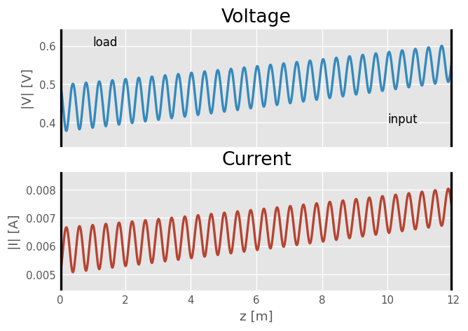
Voltage and current are plotted below against the transmission line length (pay attention to the sign of \(d\) in the voltage and current propagation: as we go from source (\(z=d\)) to the load (\(z=0\)), \(\theta\) goes in the opposite direction and should be inversed)

ds = linspace(0, d, num=1001)

thetas = - gamma*ds

v1 = np.full_like(ds, V_in)
i1 = np.full_like(ds, I_in)

v2, i2 = rf.voltage_current_propagation(v1, i1, Z_0, thetas)

/home/docs/checkouts/readthedocs.org/user_builds/scikit-rf/envs/latest/lib/python3.10/site-packages/numpy/core/numeric.py:407: ComplexWarning: Casting complex values to real discards the imaginary part
  multiarray.copyto(res, fill_value, casting='unsafe')

fig, (ax_V, ax_I) = plt.subplots(2, 1, sharex=True)
ax_V.plot(ds, abs(v2), lw=2)
ax_I.plot(ds, abs(i2), lw=2, c='C1')
ax_I.set_xlabel('z [m]')
ax_V.set_ylabel('|V| [V]')
ax_I.set_ylabel('|I| [A]')


ax_V.axvline(0, c='k', lw=5)
ax_I.axvline(0, c='k', lw=5)
ax_V.text(d-2, 0.4, 'input')
ax_V.text(1, 0.6, 'load')
ax_V.axvline(d, c='k', lw=5)
ax_I.axvline(d, c='k', lw=5)

ax_I.set_title('Current')
ax_V.set_title('Voltage')

Text(0.5, 1.0, 'Voltage')

Using media objects for transmission line calculations

scikit-rf also provides objects representing transmission line mediums. The Media object provides generic methods to produce Network’s for any transmission line medium, such as transmission line length (line()), lumped components (resistor(), capacitor(), inductor(), shunt(), etc.) or terminations (open(), short(), load()). For additional references, please see the media documentation.

Let’s create a transmission line media object for our coaxial line of characteristic impedance \(Z_0\) and propagation constant \(\gamma\):

# if not passing the gamma parameter, it would assume that gamma = alpha + j*beta = 0 + j*1
coax_line = rf.media.DefinedGammaZ0(frequency=freq, z0=Z_0, gamma=gamma)

In order to build the circuit illustrated by the figure above, all the circuit’s Networks are created and then cascaded with the ** operator:

• transmission line of length \(d\) (from the media created above),

• a resistor of impedance \(Z_L\),

• then terminated by a short.

This results in a one-port network, which \(Z\)-parameter is then the input impedance:

ntw = coax_line.line(d, unit='m') ** coax_line.resistor(Z_L) ** coax_line.short()
ntw.z

array([[[94.79804694+29.52482706j]]])

Note that full Network can also be built with convenience functions load:

ntw = coax_line.line(d, unit='m') ** coax_line.load(rf.zl_2_Gamma0(Z_0, Z_L))
ntw.z

array([[[94.79804694+29.52482706j]]])

or even more directly using or delay_load:

ntw = coax_line.delay_load(rf.zl_2_Gamma0(Z_0, Z_L), d, unit='m')
ntw.z

array([[[94.79804694+29.52482706j]]])

Determination of the propagation constant from the input impedance

Let’s assume the input impedance of a short‐circuited lossy transmission line of length d=1.5 m and a characteristic impedance of $Z_0=$100 Ohm has been measured to \(Z_{in}=40 - 280j \Omega\).

The transmission line propagation constant \(\gamma\) is unknown and researched. Let see how to deduce its value using scikit-rf:

# input data
z_in = 20 - 140j
z_0 = 75
d = 1.5
Gamma_load = -1 # short

Since we know the input impedance, we can deduce the reflection coefficient at the input of the transmission line. Since there is a direction relationship between the reflection coefficient at the load and at the input of the line:

\[\Gamma_{in} = \Gamma_L e^{- 2 \gamma d}\]

we can deduce the propagation constant value \(\gamma\) as:

\[\gamma = -\frac{1}{2d} \ln \left( \frac{\Gamma_{in}}{\Gamma_l} \right)\]

This is what the convenience function reflection_coefficient_2_propagation_constant is doing:

# reflection coefficient at input
Gamma_in = rf.zl_2_Gamma0(z_0, z_in)
# line propagation constant
gamma = rf.reflection_coefficient_2_propagation_constant(Gamma_in, Gamma_load, d)
print('Line propagation constant, gamma =', gamma, 'rad/m')

Line propagation constant, gamma = [0.03920416+1.37070847j] rad/m

One can check the consistency of the result by making the reverse calculation: the input impedance at a distance \(d\) from the load \(Z_l\):

rf.zl_2_zin(z_0, zl=0, theta=gamma * d)

array([20.-140.j])

Which was indeed the value given as input of the example.

Now that the line propagation constant has been determined, one can replace the short by a load resistance:

rf.zl_2_zin(z_0, zl=50+50j, theta=gamma * d)

array([37.90976384-20.46175538j])