How does the SWR vary along a line?

Let’s assume a 10 MHz source powering an antenna (of load \(Z_L\)) through a transmission line of length \(L\). Depending on the location of the SWR-meter, what does one would read?

This notebook is inspired from the reference: “Facts About SWR, Reflected Power, and Power Transfer on Real Transmission Lines with Loss” by Steve Stearns given at ARRL Pacificon Antenna Seminar in 2010.

Let solve this question using scikit-rf. But first, the traditional Python imports:

%matplotlib inline

import matplotlib.pyplot as plt
import numpy as np
import skrf as rf

rf.stylely()

Lossless lines

Let’s start with a lossless line of propagation constant \(\gamma=j\beta\) and characteristic impedance \(z_0=50\Omega\) (real).

freq = rf.Frequency(10, unit='MHz', npoints=1)

# load and line properties
Z_L = 75  # Ohm
Z_0 = 50  # Ohm
L = 50  # m

# propagation constant
beta = freq.w/rf.c
gamma = 1j*beta

Below we calculate the SWR of the line as a function of \(z\) the line length measured from the load (\(z=0\) at the load, \(z=L\) at the source).

z = np.linspace(start=L, stop=0, num=301)
SWRs = rf.zl_2_swr(z0=Z_0, zl=rf.zl_2_zin(Z_0, Z_L, gamma*z))

fig, ax = plt.subplots()
ax.plot(z, SWRs, lw=2)
ax.set_xlabel('z [m]')
ax.set_ylabel('SWR')
ax.set_title('SWR along the (lossless) line')
ax.invert_xaxis()
ax.axvline(0, lw=8, color='k')
ax.axvline(L, lw=8, color='k')
ax.annotate('Load', xy=(0, 1.55), xytext=(10, 1.575),
            arrowprops=dict(facecolor='black', shrink=0.05),
            )
ax.annotate('Source', xy=(50, 1.55), xytext=(40, 1.575),
            arrowprops=dict(facecolor='black', shrink=0.05),
            )

Text(40, 1.575, 'Source')

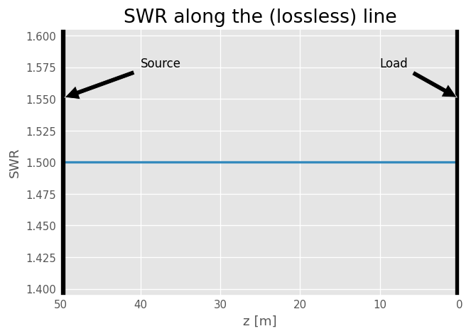
As expected, the SWR is the same everywhere along the line as the forward and backward wave amplitudes are also the same along the line.

Lossy Lines

Let’s take the previous example but this time on a lossy line. The line is defined with a propagation constant \(\gamma=\alpha + j\beta\) :

alpha = 0.01  # Np/m. Here a dummy value, just for the sake of the example
gamma = alpha + 1j*beta

z = np.linspace(0, L, num=101)
SWRs = rf.zl_2_swr(z0=Z_0, zl=rf.zl_2_zin(Z_0, Z_L, gamma*z))

fig, ax = plt.subplots()
ax.plot(z, SWRs, lw=2)
ax.set_xlabel('z [m]')
ax.set_ylabel('SWR')
ax.set_title('SWR along the (lossy) line')
ax.invert_xaxis()
ax.axvline(0, lw=8, color='k')
ax.axvline(L, lw=8, color='k')
ax.annotate('Load', xy=(0, 1.15), xytext=(10, 1.2),
            arrowprops=dict(facecolor='black', shrink=0.05),
            )
ax.annotate('Source', xy=(50, 1.4), xytext=(40, 1.5),
            arrowprops=dict(facecolor='black', shrink=0.05),
            )

Text(40, 1.5, 'Source')

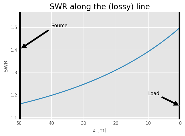
For a lossy line, the SWR is maximum at the load and decreases to be minimum at the source side.

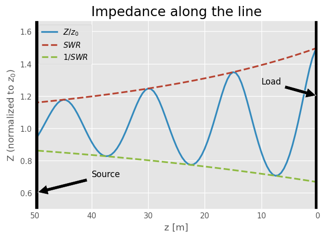
Let’s see how the impedance varies along the line:

Zins = rf.zl_2_zin(Z_0, Z_L, gamma*z)

fig, ax = plt.subplots()
ax.plot(z, np.abs(Zins/Z_0), lw=2, label='$Z/z_0$')
ax.plot(z, SWRs, lw=2, ls='--', label=r'$SWR$')
ax.plot(z, 1/SWRs, lw=2, ls='--', label=r'$1/SWR$')

ax.set_xlabel('z [m]')
ax.set_ylabel('Z (normalized to $z_0$)')
ax.set_title('Impedance along the line')
ax.invert_xaxis()
ax.axvline(0, lw=8, color='k')
ax.axvline(L, lw=8, color='k')
ax.annotate('Load', xy=(0, 1.2), xytext=(10, 1.275),
            arrowprops=dict(facecolor='black', shrink=0.05),
            )
ax.annotate('Source', xy=(50, 0.6), xytext=(40, 0.7),
            arrowprops=dict(facecolor='black', shrink=0.05),
            )
ax.legend()

<matplotlib.legend.Legend at 0x7f1fa45e6410>

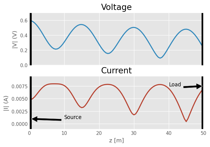
The previous result is due to the fact that voltages and currents vary along the transmission line:

V_s = 1
Z_in = rf.zl_2_zin(Z_0, Z_L, gamma*z)
# Z_s = Z_0
V_in = V_s * Z_in/(Z_0 + Z_in)
I_in = V_in/(Z_0 + Z_in)
# note that here we are going from source to load
V, I = rf.voltage_current_propagation(V_in, I_in, Z_0, gamma*z)

fig, ax = plt.subplots(2,1,sharex=True)
ax[0].plot(z, np.abs(V), lw=2)
ax[1].plot(z, np.abs(I), lw=2, color='C1')
ax[1].set_xlabel('z [m]')
ax[0].set_ylabel('|V| (V)')
ax[1].set_ylabel('|I| (A)')
ax[0].set_title('Voltage')
ax[1].set_title('Current')
[a.axvline(0, lw=8, color='k') for a in ax]
[a.axvline(L, lw=8, color='k') for a in ax]
ax[1].annotate('Load', xy=(50, 0.0075), xytext=(40, 0.0075),
            arrowprops=dict(facecolor='black', shrink=0.05))
ax[1].annotate('Source', xy=(0, 0.001), xytext=(10, 0.001),
            arrowprops=dict(facecolor='black', shrink=0.05))

Text(10, 0.001, 'Source')