Time domain reflectometry, measurement vs simulation

This example demonstrate the use of frequency to time domain transformation by comparing measurements and simulations of a microstripline and a microstripline with stepped impedance sections.

The simulation data is generated by skrf using a simple transmission line model for connectors and each impedance section. To achieve a reasonable agreement between measured and simulated data, the dielectric permittivity as well as the connector impedance and delay are extracted by optimization. The code for the simulation and parameters optimization is given at the end of the example.

Data preparation

Setup

%matplotlib inline
import skrf
from skrf.media import MLine, DefinedAEpTandZ0
import numpy as np
from numpy import real, log, log10, sum, absolute, pi, sqrt
from scipy.optimize import minimize
import matplotlib.pyplot as plt
from IPython.display import *
skrf.stylely()

Load data into skrf

The measurement was performed the 19th February 2018 on an Anritsu MS46524B 20GHz Vector Network Analyser. The setup is a linear frequency sweep from 1MHz to 10GHz with 1MHz step, 10000 points. If bandwidth 1kHz, 0dBm output power, no smoothing, no averaging. Full two-port calibration with eCal kit.

Considerations about time resolution and range limitation to avoid alias response are at the end of this document.

#load all measurement and simulation data into a dictionary
meas = skrf.read_all_networks('tdr_measurement_vs_simulation/measurement/')
simu = skrf.read_all_networks('tdr_measurement_vs_simulation/simulation/')

DC point extrapolation

The measured and simulated data are available from 1 Mhz to 10 GHz with 1 MHz step (harmonic sweep), thus we need to extrapolate the dc point.

names = ['P1-MSL_Stepped_140-P2',
         'P1-MSL_Thru_100-P2']

meas_dc_ext = meas.copy()
simu_dc_ext = simu.copy()
for k, n in enumerate(names):
    meas_dc_ext[n] = meas_dc_ext[n].extrapolate_to_dc(kind='linear')
    simu_dc_ext[n] = simu_dc_ext[n].extrapolate_to_dc(kind='linear')

Microstripline

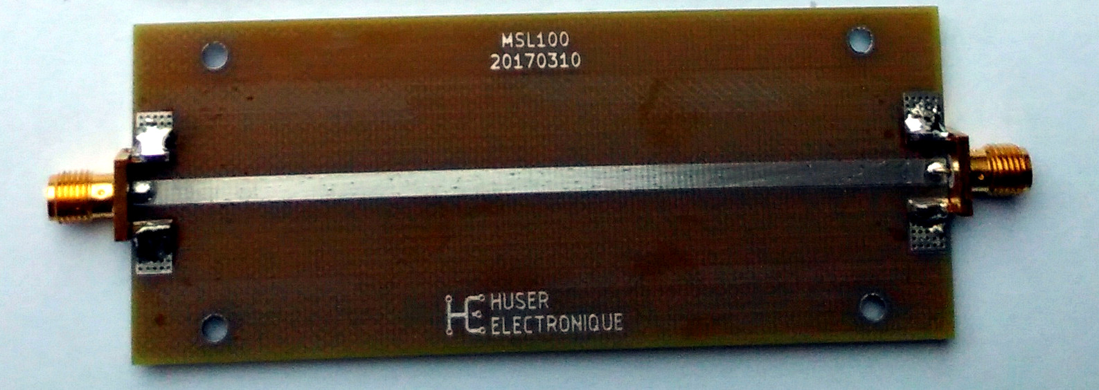
MSL_Thru_100 is a \(L1\) long, \(W1\) wide, \(T\) thick copper microstripline on a \(H\) height substrate with bottom ground plane.

Parameter	Value
\(L1\)	100mm
\(W1\)	3.0mm
\(T\)	50umm
\(H\)	1.5mm
Connector	Cinch, 142-0701-851
Substrate	FR-4

Image('tdr_measurement_vs_simulation/figures/MSL_100.jpg', width='50%')

Measurement vs simulation comparison

plt.figure()
plt.subplot(2,2,1)
plt.title('Time')
meas_dc_ext['P1-MSL_Thru_100-P2'].s11.plot_z_time_step(window='hamming', label='meas')
simu_dc_ext['P1-MSL_Thru_100-P2'].s11.plot_z_time_step(window='hamming', label='simu')
plt.xlim((-2, 3))

plt.subplot(2,2,2)
plt.title('Frequency')
meas_dc_ext['P1-MSL_Thru_100-P2'].s11.plot_s_db(label='meas')
simu_dc_ext['P1-MSL_Thru_100-P2'].s11.plot_s_db(label='simu')

plt.subplot(2,2,3)
z0 = 50
t, ymea = meas_dc_ext['P1-MSL_Thru_100-P2'].s11.step_response(window='hamming', pad=0)
ymea[ymea ==  1.] =  1. + 1e-12  # solve numerical singularity
ymea[ymea == -1.] = -1. + 1e-12  # solve numerical singularity
ymea = z0 * (1+ymea) / (1-ymea)
t, ysim = simu_dc_ext['P1-MSL_Thru_100-P2'].s11.step_response(window='hamming', pad=0)
ysim[ysim ==  1.] =  1. + 1e-12  # solve numerical singularity
ysim[ysim == -1.] = -1. + 1e-12  # solve numerical singularity
ysim = z0 * (1+ysim) / (1-ysim)
plt.xlabel('Time (ns)')
plt.ylabel('Relative error (%)')
plt.plot(t*1e9, 100*(ysim-ymea)/ymea)
plt.xlim((-2, 3))

plt.subplot(2,2,4)
delta = simu_dc_ext['P1-MSL_Thru_100-P2'].s_db[:,0,0] - meas_dc_ext['P1-MSL_Thru_100-P2'].s_db[:,0,0]
f = simu_dc_ext['P1-MSL_Thru_100-P2'].f * 1e-9
plt.xlabel('Frequency (GHz)')
plt.ylabel('Delta (dB)')
plt.plot(f, delta)
plt.ylim((-20,20))

plt.tight_layout()
plt.show()

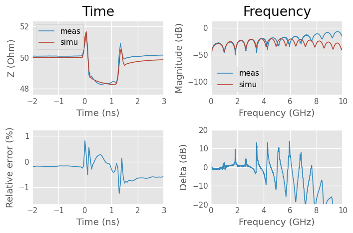
Surprisingly, the time domain results shows a very good agreement, within ±2%, while the frequency domain results exhibit a reasonable agreement only on the lower half of the frequencies.

This is because the time domain base shape is mostly impacted by the low frequency data.

There is a small offset between the time domain data, sign that the DC point is a bit different. The inductive peaks caused by the connector-to-microstripline transition are clearly visible and their simulation model agree well with measurements.

To go further, it would be possible to measure up to a bigger frequency span, thus increasing the resolution and build the dut on a more frequency stable substrate, but this would be more costly. A cross section of the transmission line could also improve the knowledge of the actual geometry, including manufacturing tolerances.

Stepped impedance microstripline

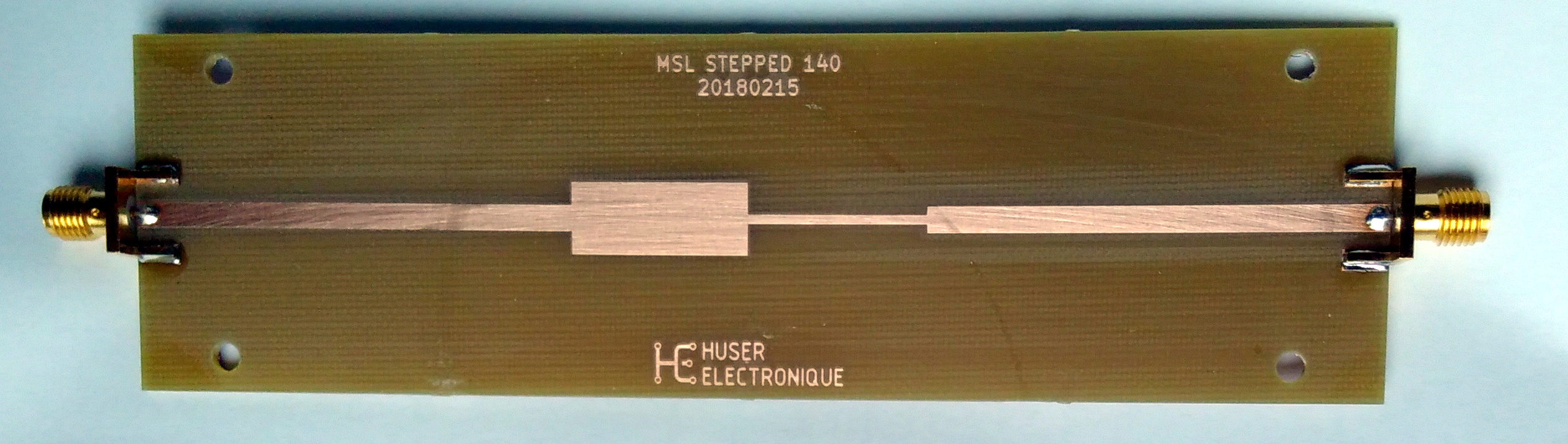
MSL_Stepped_100 is a stepped microstripline made of \(T\) thick copper on a \(H\) height substrate with bottom ground plane. The section 1, 2, 3 and 4 from the left to the right, are described with length \(Lx\) and width \(Wx\), where \(x\) is the section number.

Parameter	Value
\(L1\)	50mm
\(W1\)	3.0mm
\(L2\)	20mm
\(W2\)	8.0mm (capacitive)
\(L3\)	20mm
\(W3\)	1.0mm (inductive)
\(L4\)	50mm
\(W4\)	3.0mm
\(T\)	50umm
\(H\)	1.5mm
Connector	Cinch, 142-0701-851
Substrate	FR-4

Image('tdr_measurement_vs_simulation/figures/MSL_Stepped_140.jpg', width='75%')

Measurement vs simulation comparison

plt.figure()
plt.subplot(2,2,1)
plt.title('Time')
meas_dc_ext['P1-MSL_Stepped_140-P2'].s11.plot_z_time_step(window='hamming', label='measurement')
simu_dc_ext['P1-MSL_Stepped_140-P2'].s11.plot_z_time_step(window='hamming', label='simulation')
plt.xlim((-1, 3))

plt.subplot(2,2,2)
plt.title('Frequency')
meas_dc_ext['P1-MSL_Stepped_140-P2'].s11.plot_s_db(label='measurement')
simu_dc_ext['P1-MSL_Stepped_140-P2'].s11.plot_s_db(label='simulation')

plt.subplot(2,2,3)
z0 = 50
t, ymea = meas_dc_ext['P1-MSL_Stepped_140-P2'].s11.step_response(window='hamming', pad=0)
ymea[ymea ==  1.] =  1. + 1e-12  # solve numerical singularity
ymea[ymea == -1.] = -1. + 1e-12  # solve numerical singularity
ymea = z0 * (1+ymea) / (1-ymea)
t, ysim = simu_dc_ext['P1-MSL_Stepped_140-P2'].s11.step_response(window='hamming', pad=0)
ysim[ysim ==  1.] =  1. + 1e-12  # solve numerical singularity
ysim[ysim == -1.] = -1. + 1e-12  # solve numerical singularity
ysim = z0 * (1+ysim) / (1-ysim)
plt.xlabel('Time (ns)')
plt.ylabel('Relative error (%)')
plt.plot(t*1e9, 100*(ysim-ymea)/ymea)
plt.xlim((-2, 3))

plt.subplot(2,2,4)
delta = simu_dc_ext['P1-MSL_Stepped_140-P2'].s_db[:,0,0] - meas_dc_ext['P1-MSL_Stepped_140-P2'].s_db[:,0,0]
f = simu_dc_ext['P1-MSL_Stepped_140-P2'].f * 1e-9
plt.xlabel('Frequency (GHz)')
plt.ylabel('Delta (dB)')
plt.plot(f, delta)
plt.ylim((-10,10))

plt.tight_layout()
plt.show()

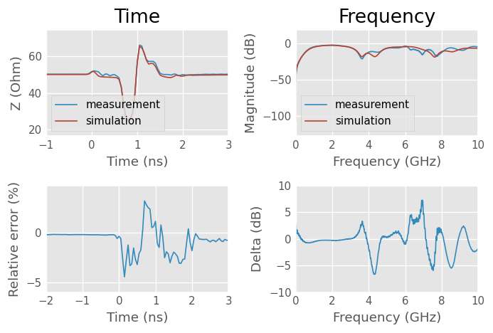
Both time domain and the frequency domain results shows a reasonable agreement, within ±5% for time domain. The frequency domain results exhibit a good agreement, within ±dB only on the lower half of the frequencies, and the upper frequencies shows better agreement than in the previous microstripline case.

An explanation to the better frequency domain agreement is that the impedance steps induce such a discontinuities that more energi is reflected back, leading to a shorter effective length and an increased accuracy (more signal).

The capacitive and inductive section of the stepped line are clearly visible and their simulation model agree well with measurements. The first connector effect is hidden by the plot scale, while the second is masked by the reflexions.

To go further, it would again be possible to measure up to a bigger frequency span, thus increasing the resolution and build the dut on a more frequency stable substrate, but this would be more costly. A cross section of the transmission line could also improve the knowledge of the actual geometry, including manufacturing tolerances.

Eventually, the stepped discontinuities could be made smaller, to produce a smaller effect on the overall measurement (each discontinuity has an influence on the following time domain signal shape).

Parameters optimization

Dielectric effective relative permittivity and loss tangent characterisation based on multiline method

Only two lines with different lengths are required for dielectric permittivity and loss tangent characterisation. Since we have measured the reflects too, we will use them instead of fake reflects. We don’t have the switch terms either, but as we only extract the dielectric permittivity and loss tangent rather that doing a real calibration, there is no problem with that.

Multiline calibration algorithm get rid of connectors effects by using multiple lengths of lines. The docstring explain that At every frequency point there should be at least one line pair that has a phase difference that is not 0 degree or a multiple of 180 degree otherwise calibration equations are singular and accuracy is very poor. These conditions will not be met with the chosen lines combination, but we will still be able to get a decent estimation of the dielectric permittivity and loss tangent.

Image('tdr_measurement_vs_simulation/figures/MSL_100.jpg', width='50%')

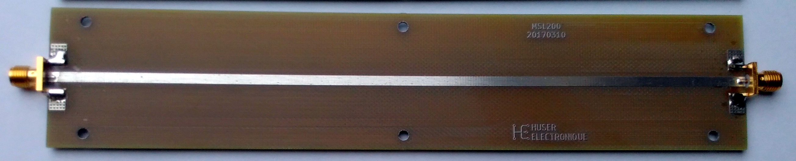
Image('tdr_measurement_vs_simulation/figures/MSL_200.jpg', width='100%')

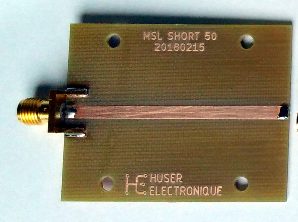
Image('tdr_measurement_vs_simulation/figures/MSL_Short_50.jpg', width='25%')

Perform NISTMultilineTRL algorithm

Discard the No switch term provided warning.

# Perform NISTMultilineTRL algorithm
line100mm = meas['P1-MSL_Thru_100-P2']
line200mm = meas['P1-MSL_Thru_200-P2']
short50mm = skrf.network.two_port_reflect(meas['P1-MSL_Short_50'], meas['P2-MSL_Short_50'])
measured  = [line100mm, short50mm, line200mm]
Grefls    = [-1]
lengths   = [100e-3, 200e-3] # in meter
offset    = [50e-3] # in meter
cal = skrf.NISTMultilineTRL(measured, Grefls, lengths, er_est=4.5, refl_offset=offset)

/home/docs/checkouts/readthedocs.org/user_builds/scikit-rf/envs/latest/lib/python3.10/site-packages/skrf/calibration/calibration.py:2775: UserWarning: No switch terms provided
  EightTerm.__init__(self,

Relative dielectric permittivity and loss tangent

The NISTMultilineTRL calibration give the frequency-dependent effective relative dielectric of the geometry, which is a mix between air and substrate relative permittivity.

Unfortunately, a single value of relative dielectric permittivity of the substrate at a given frequency is required for the microstripline media simulation, instead of the frequency-dependent effective value of the geometry we get from the calibration.

To overcome this difficult situation, the microstripline model which will be used is fitted by optimization on the calibration results in such a way the difference between the frequency-dependent effective relative dielectric permittivity of both dataset is minimised.

Additionally, a weighted contribution of the dielectric loss tangent is inserted in the optimization to minimise the difference between the measured modelled attenuation.

The optimization results are dielectric \(\epsilon_r\) and \(\tan{\delta}\) at 1 GHz and will be used in the dielectric dispersion model.

# frequency axis
freq  = line100mm.frequency
f     = line100mm.frequency.f
f_ghz = line100mm.frequency.f/1e9

# the physical dimensions of the lines are known by design (neglecting manufacturing tolerances)
W   = 3.00e-3
H   = 1.55e-3
T   = 50e-6
L     = 0.1

# calibration results to compare against
ep_r_mea = cal.er_eff.real
A_mea    = 20/log(10)*cal.gamma.real

# starting values for the optimizer
A     = 0.0
f_A   = 1e9
ep_r0 = 4.5
tanD0 = 0.02
f_epr_tand  = 1e9
x0 = [ep_r0, tanD0]

# function to be minimised
def model(x, freq, ep_r_mea, A_mea, f_ep):
    ep_r, tanD = x[0], x[1]
    m = MLine(frequency=freq, Z0=50, w=W, h=H, t=T,
            ep_r=ep_r, mu_r=1, rho=1.712e-8, tand=tanD, rough=0.15e-6,
             f_low=1e3, f_high=1e12, f_epr_tand=f_ep,
             diel='djordjevicsvensson', disp='kirschningjansen')
    ep_r_mod = m.ep_reff_f.real
    A_mod = m.alpha * 20/log(10)
    return sum((ep_r_mod - ep_r_mea)**2)  + 0.1*sum((A_mod - A_mea)**2)

# run optimizer
res = minimize(model, x0, args=(freq, ep_r_mea, A_mea, f_epr_tand),
               bounds=[(4.0, 5.0), (0.001, 0.1)])

# get the results and print the results
ep_r, tanD = res.x[0], res.x[1]
print('epr={:.3f}, tand={:.4f} at {:.1f} GHz.'.format(ep_r, tanD, f_epr_tand * 1e-9))

# build the corresponding media
m = MLine(frequency=freq, Z0=50, w=W, h=H, t=T,
         ep_r=ep_r, mu_r=1, rho=1.712e-8, tand=tanD, rough=0.15e-6,
         f_low=1e3, f_high=1e12, f_epr_tand=f_epr_tand,
         diel='djordjevicsvensson', disp='kirschningjansen')

/home/docs/checkouts/readthedocs.org/user_builds/scikit-rf/envs/latest/lib/python3.10/site-packages/skrf/media/mline.py:276: RuntimeWarning: Conductor loss calculation invalid for lineheight t (5e-05)  < 3 * skin depth (6.585246128681408e-05)
  self.alpha_conductor, self.alpha_dielectric = self.analyse_loss(

epr=4.450, tand=0.0174 at 1.0 GHz.

Calibration based values are plotted against modelled value as a sanity check.

plt.figure()
plt.subplot(2,2,1)
plt.xlabel('Frequency [GHz]')
plt.ylabel('$\epsilon_{r,eff}$')
plt.plot(f_ghz, ep_r_mea, label='measured')
plt.plot(f_ghz, m.ep_reff_f.real, label='model')
plt.legend()

plt.subplot(2,2,2)
plt.xlabel('Frequency [GHz]')
plt.ylabel('A (dB/m)')
plt.plot(f_ghz, A_mea, label='measured')
A_mod = 20/log(10)*m.alpha
plt.plot(f_ghz, A_mod, label='model')
plt.legend()

plt.subplot(2,2,3)
plt.xlabel('Frequency [GHz]')
plt.ylabel('$\epsilon_{r,eff}$ error [%]')
rel_err = 100 * ((ep_r_mea - m.ep_reff_f.real)/ep_r_mea)
plt.plot(f_ghz, rel_err)
plt.ylim((-2,2))

plt.subplot(2,2,4)
plt.xlabel('Frequency [GHz]')
plt.ylabel('$A$ error [%]')
rel_err = 100 * ((A_mea - A_mod)/A_mea)
plt.plot(f_ghz, rel_err)
plt.ylim((-20,10))

plt.tight_layout()
plt.show()

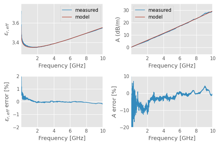
The agreement between measurements and the model seems very reasonable. Relative error of \(\epsilon_{r,eff}\) stay within ±1% outside very low frequencies and relative error of \(A\) is kept between ±10% on most of the range. Considering the shape of \(A\), it is not possible to do much better with this model.

Connector effect characterization

The NISTMultilineTRL calibration coefficients contain information about the connector characteristics, which is corrected by the calibration.

These coefficients can be used to fit a connector model based on a transmission line section.

Delay and attenuation

# extract connector characteristic from port 1 error coefficients
conn = skrf.error_dict_2_network(cal.coefs, cal.frequency, is_reciprocal=True)[0]

Estimate connector delay with linear regression on unwrapped phase.

# connector delay estimation by linear regression on the unwrapped phase
xlim = 9000 # used to avoid phase jump if any
phi_conn = (np.angle(conn.s[:xlim,1,0]))
z = np.polyfit(f[:xlim], phi_conn, 1)
p = np.poly1d(z)
delay_conn = -z[0]/(2*np.pi)
print('Connector delay: {:.1f} ps'.format(delay_conn * 1e12))

Connector delay: 41.6 ps

Build connector model and compare it against calibration extracted data.

mc = DefinedAEpTandZ0(m.frequency, ep_r=1, tanD=0.02, Z0=50,
                              f_low=1e3, f_high=1e18, f_ep=f_epr_tand, model='frequencyinvariant')

Z0_conn = 50.0 # the actual connector characteristic impedance will be tuned later
left = mc.line(delay_conn, 's', z0=Z0_conn)
check = mc.thru() ** left ** mc.thru()

plt.figure()
plt.subplot(2,1,1)
conn.plot_s_deg(1, 0, label='measured')
check.plot_s_deg(1, 0, label='model')
plt.ylabel('phase (rad)')
plt.legend()

plt.subplot(2,1,2)
conn.plot_s_db(1, 0, label='Measured')
check.plot_s_db(1, 0, label='Model')
plt.xlabel('Frequency (GHz)')
plt.ylabel('Insertion Loss (dB)')
plt.legend()

plt.tight_layout()
plt.show()

/tmp/ipykernel_6163/1413003635.py:1: DeprecationWarning: Use of `Z0` in DefinedAEpTandZ0 initialization is deprecated.
`Z0` has no effect. Use `z0` instead
`Z0` will be removed in version 1.0
  mc = DefinedAEpTandZ0(m.frequency, ep_r=1, tanD=0.02, Z0=50,

/home/docs/checkouts/readthedocs.org/user_builds/scikit-rf/envs/latest/lib/python3.10/site-packages/skrf/mathFunctions.py:268: RuntimeWarning: divide by zero encountered in log10
  out = 20 * npy.log10(z)

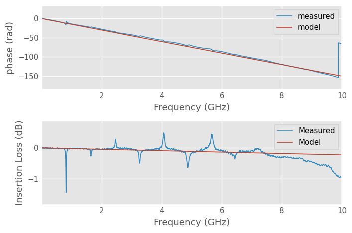
Comparison of connector model characteristics against calibration results shows a reasonable agreement. Calibration results exhibit some glitches that do not correspond to the expected physical behavior. They are caused by the calibration being close to singular due to the thru and line phase being a multiple of 180 degrees. Accuracy could be enhanced by feeding more distinct lines to the algorithm, but these are not manufactured yet.

Characteristic impedance

We now have estimated connector delay and attenuation, but what about the characteristic impedance? This value is required to properly parametrize the transmission line section model.

Optimization is used to find the characteristic impedance that minimize the difference between modelled and measured return loss.

s11_ref = conn.s[:,0,0]
x0 = [Z0_conn]

# function to be minimised
def model2(x, mc, delay_conn, s11_ref):
    Z0_mod = x[0]
    conn_mod = mc.line(delay_conn, 's', z0=Z0_mod)
    check = mc.thru(z0 = 50.) ** conn_mod ** mc.thru(z0 = 50.)
    s11_mod = check.s[:,0,0]

    return sum(absolute(s11_ref-s11_mod))

# run optimizer
res = minimize(model2, x0, args=(mc, delay_conn, s11_ref),
               bounds=[(20, 100)])

# get the results and print the results
Z0_conn = res.x[0]
print('Z0_conn={:.1f} ohm.'.format(Z0_conn))

Z0_conn=52.9 ohm.

The modelled results are plotted against the calibration data, as a sanity check.

conn_mod = mc.line(delay_conn, 's', z0=Z0_conn)
check = mc.thru(z0 = 50.) ** conn_mod ** mc.thru(z0 = 50.)

plt.figure;
plt.subplot(2,1,1)
conn.plot_s_db(0,0, label = 'measured')
check.plot_s_db(0,0, label = 'model')


plt.subplot(2,1,2)
plt.plot(check.f*1e-9, (check.s_db[:,0,0]-conn.s_db[:,0,0]))
plt.ylabel('Delta (dB)')
plt.xlabel('Frequency (GHz)')

plt.tight_layout()
plt.show()

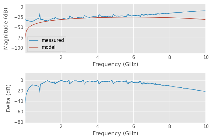
The delta in dB is quite big in low and high frequencies, but we will see when comparing measurement and simulation that the time domain reflectometry results are very decent with this value. The connector effects inductive peaks are well rendered in the case of the microstripline.

Simulation

Frequency axis

freq = skrf.F(1,10e3,10000, 'mhz')

Media sections with different geometries

# 50 ohm segment
MSL1 = MLine(frequency=freq, z0_port=50, w=W, h=H, t=T,
        ep_r=ep_r, mu_r=1, rho=1.712e-8, tand=tanD, rough=0.15e-6,
        f_low=1e3, f_high=1e12, f_epr_tand=f_epr_tand,
        diel='djordjevicsvensson', disp='kirschningjansen')

# Capacitive segment
MSL2 = MLine(frequency=freq, z0_port=50, w=8.0e-3, h=H, t=T,
        ep_r=ep_r, mu_r=1, rho=1.712e-8, tand=tanD, rough=0.15e-6,
        f_low=1e3, f_high=1e12, f_epr_tand=f_epr_tand,
        diel='djordjevicsvensson', disp='kirschningjansen')

# Inductive segment
MSL3 = MLine(frequency=freq, z0_port=50, w=1.0e-3, h=H, t=T,
        ep_r=ep_r, mu_r=1, rho=1.712e-8, tand=tanD, rough=0.15e-6,
        f_low=1e3, f_high=1e12, f_epr_tand=f_epr_tand,
        diel='djordjevicsvensson', disp='kirschningjansen')

# Connector transmission line media with guessed loss
MCON = DefinedAEpTandZ0(m.frequency, z0_port=50, ep_r=1, tanD=0.025, z0=Z0_conn,
        f_low=1e3, f_high=1e18, f_ep=f_epr_tand, model='frequencyinvariant')

Simulated devices under test

# SMA connector
conn_sma  = MCON.line(delay_conn, 's')


# microstripline
thru_simu = conn_sma ** MSL1.line(100e-3, 'm') ** conn_sma
thru_simu.name = 'P1-MSL_Thru_100-P2'

# stepped impedance microstripline
step_simu = conn_sma \
           ** MSL1.line(50e-3, 'm') \
           ** MSL2.line(20e-3, 'm') \
           ** MSL3.line(20e-3, 'm') \
           ** MSL1.line(50e-3, 'm') \
           ** conn_sma
step_simu.name = 'P1-MSL_Stepped_140-P2'

# write simulated data to .snp files
write_data = False
if write_data:
    step_simu.write_touchstone(dir='tdr_measurement_vs_simulation/simulation/')
    thru_simu.write_touchstone(dir='tdr_measurement_vs_simulation/simulation/')

Notes

Time resolution

After DC point extrapolation, and neglecting the effect of windowing, the time resolution of measurement is \begin{equation*} Resolution = \frac{1}{f_{span}} \end{equation*}

where \(Resolution\) is the resolution in s and \(f_{span}\) is the frequency span in Hz.

In our case, with \(f_{span} = 10 \mskip3mu\mathrm{[GHz]}\) \begin{equation*} Resolution \approx \frac{1}{10^{10}} \approx 100 \quad \mathrm{[ps]} \end{equation*}

With an effective relative dielectric permittivity of about 3.5, this give following physical resolution: \begin{equation*} Resolution_{meter} = \frac{Resolution \dot{} c_0}{\sqrt{\epsilon{}_r}} \approx \frac{10^{-10} \dot{} 3\dot{}10^8}{\sqrt{3.5} } \approx 16 \quad \mathrm{[mm]} \end{equation*}

We will use reflexion measurement, so the actual range is divided by two, because the signal goes back and forth. Thus, the approximate distance resolution on our device under test will be 8mm. The discontinuities on the stepped impedance microstripline and the connector effects shall be well visible.

Measurement range limitation to avoid alias response

The measurement range should be set in such a way the true response of the device is seen without repetitions (alias).

\begin{equation*} Range = \frac{c_0}{\sqrt{\epsilon{}_r} \dot{} \Delta{}_f} \end{equation*}

Where \(Range\) is the range in m, \(c_0\) the speed of light in m/s, \(\Delta{}_f\) the frequency step in Hz and \(\epsilon{}_r\) is the effective relative permittivity constant of the device under test.

With the given measurement setup and considering \(\Delta{}_f = 1 \mskip3mu\mathrm{[MHz]}\), worst case \(\epsilon{}_r \approx 5.0\), the range is \begin{equation*} Range \approx \frac{3\dot{}10^8}{\sqrt{5} \dot{} 10^6} \approx 134 \quad \mathrm{[m]} \end{equation*} Relative dielectric permittivity for FR-4 is approximately 5.0, the effective \(\epsilon{}_r\) of microstripline geometry will be smaller because of the air on top, which give a safety margin, the range being underevaluated.

We will use reflexion measurement, so the actual range is divided by two, because the signal goes back and forth. However, our longest device being 200mm long, we can just quietly forget aliasing.